Computation - Operations Management/Industrial Engineering

Computation

Inventory Analysis

Deterministic-No Shortages

Deterministic- Shortages

	Inventory Analysis
	Deterministic Models - No Shortages

Creating a Model

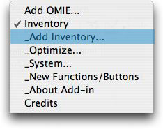
To create a model choose Add Inventory from the menu. The dialog below is presented.

Near the top of the dialog we see the address of the worksheet cell where the top of the inventory definition will be placed. The Name entered here is used for naming ranges. The Time Interval defines the interval used for all rates and time intervals. The Replications box allows several inventories to be simultaneously created.

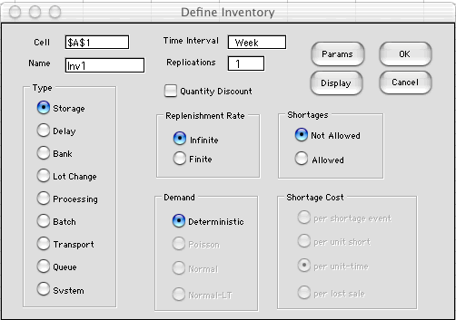
Buttons on the dialog determine the type of model to be created. The Type buttons determine what kind of inventory is to be modeled. The Storage inventories are discussed on the majority of pages in this section of the site. The other options are for WIP and are discussed on the Work-in-Progress and Systems pages. The Replenishment Rate buttons determine if the inventory is to be replenished by a finite rate process or whether the entire inventory quantity arrives instantaneously (at an infinite rate). The former case is appropriate if a manufacturing process provides materials to the inventory and the latter case is appropriate when a batch delivery occurs.

Buttons under the Shortages label determine if shortages are allowed and their effect on the system. We illustrate the no shortages case here.

When the Quantity Discount button is checked and more than one replication is specified, the add-in constructs a model that determines the optimum when discounts are offered for larger purchases.

The Demand box determines if the product is demanded from the inventory at a deterministic rate or whether it is governed by a probability distribution. We illustrate the deterministic case here and will discuss the stochastic options later.

The Shortage Cost area specifies how shortages affect the cost of the inventory. Since no shortages are allowed for this example, the buttons are disabled.

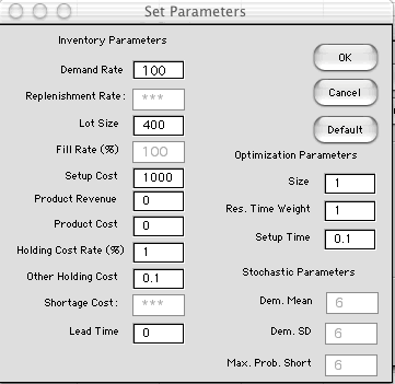
The Params button presents a new dialog, illustrated below. The dialog allows direct entry of the parameters associated with the inventory model. The example shows the default values. The boxes related to stochastic parameters and shortages are not available because the current model is deterministic and allows no shortages. Parameters entered with this dialog are placed on the Excel worksheet. They may be changed arbitrarily once the model is created, so it is really unnecessary to set the parameters here.

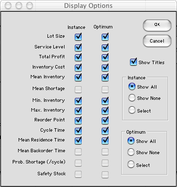
The Display button on the Inventory definition dialog presents another dialog with buttons that determine which results are presented on the worksheet. In some cases the student may wish to show only a few. The boxes under Instance will add worksheet rows that compute the items for design variables specified by the student. Boxes under Optimum will add rows that compute the optimum results.

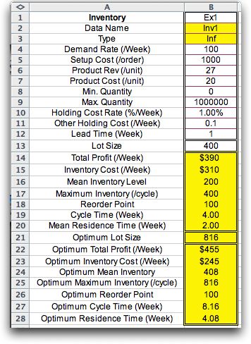
The figure below shows the entries placed on the worksheet by the add-in. Although the display can appear anywhere on the worksheet the example is placed in columns A and B. The titles are in column A and the data and results are in column B. Four kinds of information appear in the display. They are separated by the double outlines.

Parameters
The first part of the display holds the parameters of the model. The number of rows used depends on type of model. For the example the parameters are in rows 1 through 12. The first entry is set by the user to identify the inventory. The other parameters may be changed except the Data Name and Type. The data name is used to name cells on the worksheet. The type is used by the program and should not be changed. All numeric parameters are to be nonnegative.

Instance Variables
For the example there is only instance variable the lot size in cell B13. For models involving shortages we also specify the fill rate. For stochastic models there is an entry for the reorder point.

Instance Results
These are all computed by functions provided by the add-in. Cells B14 through B29 are colored yellow to indicate that their contents should not be changed. The cells hold functions that depend on the parameters and the instance variables. Changing the instance variables causes the formula results to change.

Optimum Results
These are computed in cells B22 though B28. Again, the yellow color indicates that the cells contain formulas and should not be changed. The optimum results depend on the parameters. Changing the parameters will result in new optimum results.

On this and the following pages, we consider the several models that are available and explain the meaning of the parameters and results for each model.

Infinite Replenishment Rate and No Shortages

The first model considered is illustrated by the figure below which shows the variation of the inventory level with time.

The figure shows time on the horizontal axis and inventory level on the vertical axis. We begin at time 0 with an order arriving. The amount of the order is the lot size, q. The lot is delivered all at one time causing the inventory to shoot from 0 to q instantaneously. Material is withdrawn from inventory at a continuous demand rate, D, measured in units per time interval. We are assuming that the material is withdrawn in a continuous fashion, rather than in discrete units, so we show the inventory level declining as a straight line. After an amount of time q/D, the inventory is depleted. At that time another order of size q arrives and the cycle repeats.

The inventory pattern shown in the figure is obviously an abstraction of reality in that we expect no real system to operate exactly as shown. The abstraction does provide an estimate of the optimum lot size, called the economic order quantity (EOQ), and related quantities. We consider alternatives to those assumptions later on these pages.

Notation

Parameters

The models depend on a variety of parameters. This section lists the factors that are important in making decisions related to inventories and establishes some of the notation that is used in this section. Dimensional analysis is sometimes useful for modeling inventory systems, so we provide the dimensions of each factor. Additional model dependent notation is introduced later.

Inventory
The name appearing in B1 is the name assigned on the dialog. The contents of B1 may be changed to reflect the product under consideration.

Data Name
The name appearing in B2 is used to name arrays on the worksheet. No other inventory in the workbook can be assigned this name.

Type
The type is determined by the options on the dialog. In this case they indicate that inventory has an infinite replenishment rate. Do not change the Type that has been assigned by the add-in.

Demand rate (D): This is the constant rate at which the product is withdrawn from inventory. (units / time)

Setup cost (A): A common assumption is that the cost of placing an order cost consists of a fixed cost, that is independent of the amount ordered, and a variable cost that depends on the amount ordered. The fixed cost is called the setup cost and given in ($).

Product revenue (R): This is the unit revenue obtained when the product is sold. This used for the profit model, but not for the inventory cost model. ($/unit).

Product cost (C): This is the unit cost of purchasing the product as part of an order. The value is used in the profit calculation. The value of C is used to measure the investment in the item as it relates to holding cost. ($/unit)

Min Quantity (q_min): This places a lower bound on the order quantity (unit)

Max Quantity (q_min): This places an upper bound on the order quantity (unit)

Holding cost rate (i): This is discount rate or interest rate used to compute the inventory holding cost. The holding cost usually includes the lost investment income caused by having the asset tied up in inventory. This is not a real cash flow, but it is an important component of the cost of inventory. If C is the unit cost of the product, this component of the cost is Ci, where i is the holding rate. (%/unit-time)

Other holding cost: The holding cost may also include the cost of storage, insurance, and other factors that are proportional to the amount stored in inventory and the time an item remains in inventory. In the following we use H as the holding cost per unit including both the lost investment income and other holding cost. ($/unit-time)

Lead time (L): This is time interval between when an order is placed and when the inventory is replenished. (time)

Results

We repeat the computed results for the example. The figure showing a single cycle of the inventory is shown at the right.

Lot Size (q): This is the fixed quantity received at each inventory replenishment. The instance results depend directly on this quantity. (units)

Total Profit: This is the product revenue less the product cost less the cost the cost of running the inventory. In some cases, the optimum inventory policy does not depend on product cost and revenue, so we often set these factors to zero. Then the profit will be simply the negative of the inventory cost, as it is here.($/time)

Inventory Cost (z) This is the cost associated with having an inventory. It includes the ordering cost, holding cost and costs related to shortages. Traditionally we select a policy to minimize T.($/time).

Mean Inventory Level: This is the average level of inventory over time. For this case it is q/2.(units)

Maximum Inventory Level: For this case it is q. (units). We do not show the minimum since it is always 0 for the deterministic system with no loses.

Reorder Point: This is the inventory level that signals that an order for replenishment should be made. For this system, it is the inventory level for a time L before the inventory reaches 0.

Cycle time: The time between successive orders. For this case it is q/D.

Mean residence time: This is average time a unit spends in the inventory. By Little's law it is: (mean inventory level)/D.

Optimum Results
The optimum results are similar to the instance results except they use the optimum order quantity and fill rate (only the order quantity is relevant here).

Finite Replenishment Rate and No Shortages

The model with finite replenishments is illustrated below. Rather than arrive instantaneously, the lot is assumed to arrive continuously at a rate P. This situation arises when a production process feeds the inventory and the process operates at the rate P. Of course P must be greater than the demand rate D.

A more detailed picture of a cycle illustrates some important points.The maximum inventory level never reaches q because material is withdrawn at the same time it is being replenished. Replenishment takes place at the beginning of the cycle. After the full amount q is delivered, the inventory is drawn down at the demand rate D until it reaches 0 at the end of the cycle. This model requires the single new parameter P.

To create an example for this type, click the Finite button and enter a replenishment rate.

The results are shown at the left. The only new parameter is the replenishment rate of 200, twice the demand rate. Of course, the replenishment rate must greater than the demand rate to obtain a feasible solution. With the same parameters as the infinite replenishment case, we expect the finite case to have a larger optimum lot size. This is substantiated by the results.

The reorder point has a somewhat different definition than for the infinite replenishment case. The reorder point is measured with respect to inventory position. This is equal to on-hand inventory plus the amount on order. The reorder point then refers to a unique time in each cycle.

These models change when shortages are allowed. These results are on the next page.