|
|
|
|
Inventory
Theory
|
 |
-
Deterministic/Infinite Replenishment/No
Shortages
|
| |
 |
In this section we
consider an isolated inventory in which external demanders remove
items from the inventory and external suppliers replenish the
inventory. Rather than demand occurring in a random and uncertain
manner, we assume that items are withdrawn from the inventory
at a continuous rate. Replenishments to the inventory are of
a fixed size q, called the lot size The time between
when a replenishment is requested and when the amount enters
the inventory is called the lead-time. We assume that the lead-time
is zero or a constant. The resulting behavior of the inventory
is shown in Fig. 1. We use this deterministic model of the system
to explain some of the notation associated with inventory. Because
of its simplicity, we are able to find an optimal solution to
this deterministic model. The solution specifies the optimum
lot size. This appears in many texts on operations management
with the name economic order quantity or EOQ. |
Infinite Replenishment Rate and
No Shortages |
| |
The first model considered
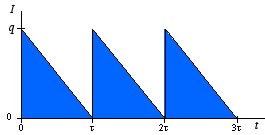
is illustrated by the figure below which shows the variation
of the inventory level with time.

Figure 1. Inventory with Infinite Replenishment rate
and no shortages
|
The figure shows time on the horizontal axis
and inventory level on the vertical axis. We begin at time
0 with an order arriving. The amount of the order is the lot
size, q. The lot is delivered all at one time
causing the inventory to shoot from 0 to q instantaneously.
Material is withdrawn from inventory at a continuous demand
rate, D, measured in units per time interval. We are
assuming that the material is withdrawn in a continuous fashion,
rather than in discrete units, so we show the inventory level
declining as a straight line. After an amount of time q/D,
the inventory is depleted. At that time another order of size q arrives
and the cycle repeats. The cycle time is  . .
The inventory pattern shown in the figure is
obviously an abstraction of reality in that we expect no real
system to operate exactly as shown. The abstraction does provide
an estimate of the optimum lot size, called the economic
order quantity (EOQ), and related quantities. We consider
alternatives to those assumptions on later pages. |
Formulas for Instance Results |
| |


Click buttons to see the notation
|
Here
we derive the formulas for the results for an instance.
An instance is defined by a collection of inventory parameters
and a value for the lot size q. Click the buttons
on the left for a description of the notation for parameters
and results.
These formulas are implemented in the Inventory add-in. |
|
|
To construct a mathematical
model describing the economic costs or profits associated with
the inventory system, we show the cash flows below. This figure
is a mixed representation of discrete as well as continuous
cash flows. The arrows represent amounts paid or received at
points in time. The areas represent continuous cash flows given
by rates. Amounts appearing above the 0 axis are revenues, while
amounts below are expenditures or costs.
The table below shows the various revenue and cost components
and their respective cost rates. In all of the following, we
assume that the parameters are nonnegative and that q
> 0.
| Item |
Amount during a cycle |
Cost or revenue rate |
Ordering Cost
In each cycle an order is placed for
the quantity q
|
A |
|
| Product Cost |
Cq |
|
| Holding Cost for Product
in Inventory |
Linearly varies from Hq
to 0 in each cycle |
|
Revenue from product Sales |
Rq |
RD |
For this model there is a single decision variable that is
the lot size or the replenishment, q. All other quantities
are a function of q. The inventory cost is a strictly
convex function of q, so there is a unique global minimum
with respect to q.
Additional quantities associated with the inventory policy
are derived below.

When the lead time is greater than the
cycle time, an order for replenishment must be placed
more than one cycle before the order is delivered. The
add-in performs this more complicated computation.
|
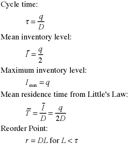
The measures are computed below for the example using a lot
size of 400 units. This is called an instance of the inventory
model. The figure shows a single cycle of the inventory pattern.
|
Optimum Policy |
| |
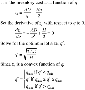
For determination of the optimum
lot size q*, the unit revenue and unit cost can be
neglected and we write the expression for the cost rate for
operating the inventory.


Since the second derivative is positive
for positive parameters, the inventory cost function
is convex and the solution for q* is a global
minimum.
|
When q* is between the minimum and maximum lot sizes,
the inventory measures with the optimum lot size are found by
substituting q* into the instance formula.
At the optimum, the holding cost is equal to the setup cost.
We see that optimal inventory cost is a concave function of
product flow through the inventory, indicating that there is
an economy of scale associated with the flow through inventory.
The optimal lot size increases with increasing setup cost and
flow rate and decreases with increasing holding cost.
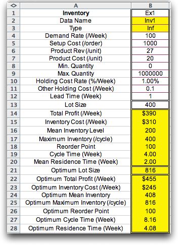
The table below shows the parameters and instance results as
well as the results for the optimum lot size (q*= 816).

|
| |
|
|


