| Infinite Replenishment
Rate and Backorders |
| |
In these
models, we allow the inventory to go to 0 some time before replenishment.
There are two assumptions regarding the response of a customer
to the unavailable item. The first response is that the customer
will accept later delivery. This is called a backorder. We provide
three cost models for the backorder case:
- There is an expense for each cycle in which a backorder
occurs. This cost is independent of the number of backorders.
The expense is measured in $.
- There is an expense for each backordered item. This cost
is independent of the time the customer must wait for delivery.
The expense is measured in $/unit.
- The expense for each item is proportional to the time the
customer must wait. For a particular cycle the total cost
is proportional to the integral of the shortage amount during
the cycle. The expense is measured in $/unit-time.
The figure below illustrates on-hand inventory
in blue and backordered quantities in red.
Since replenishments are instantaneous, backordered
items are delivered at the time of replenishment and these items
do not remain in inventory. We signify backorders as a negative
inventory, so the minimum inventory is a negative number. The
difference between the minimum and maximum inventory is the
lot size. |
Notation |
| |
When shortages are
allowed, several new quantities must be defined and several
reinterpreted.
• Backorder cost: When a customer seeks the product and
finds the inventory empty, the demand can either go unfulfilled
or be satisfied later when the product becomes available. The
former case is called a lost sale, and the latter is called
a backorder. We consider the lost sales cost later. The total
backorder cost depends on the measured adopted for backorder
cost.
• Backorder level: This is the average level of backorders
over time. It is the average area of the red areas in the figure
above.
• Fill Rate(v): This is the proportion of the
customers served directly from the inventory. The proportion
of the customers who must wait for a backordered item is 1 -
v. We use this factor as a design variable when shortages
are allowed. For the backordered case the service level is I_Max/q.
• Maximum inventory level (I_Max): Many books
call this quantity the order level. When backorders are not
allowed, this quantity is the same as q. When backorders
are allowed, it is less than q. (units)
• Minimum inventory level (I_Min=I_Max-q): When
backorders are not allowed, this quantity is 0. With
backorders its absolute value is the level of maximum number
of backordered units. (units)
• Mean Residence Time: This is the time a remains in
inventory, given that it is placed in inventory. With shortages,
not all units appear in inventory. Those units that are backordered,
go to the customer as soon as they are available. For the infinite
replenishment rate case, this is when an order arrives. We compute
the mean residence time using Little's law by dividing the average
inventory level by the rate of items entering inventory. This
rate is D(1 - v).
• Mean Backorder Time: When an item is backordered, a
customer must wait for a period of time before the backorder
is satisfied. Again we use Little's law. For the mean backorder
time, we divide the average backorder level by the rate of items
being backordered. |
Single Cycle |
| |
|
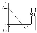
The results of the analysis
depend on the lot size and the service level. The figure
shows that the maximum inventory is the same as the order
level. In addition to the other results computed for
the no-shortages case we now can compute:
- Minimum inventory level: This is vq - q.
- Maximum inventory level: This is vq.
|
|
The Inventory Model |
| |
 |
As before, we create a model
by selecting Add Inventory from the menu. We select
Allowed from the Shortages frame on the
dialog. We select per unit-time as the Shortage
Cost measure. |
|
The results for this case
using a backorder cost of $2 per unit-week is shown at
the left. For the evaluation of an instance we choose
a lot size of 400 and a service level of 90%.
The optimum lot size is greater, 876, and the optimum
fill rate is 86.96%. The optimum solution balances ordering,
inventory and backorder costs. |
|
Infinite Replenishment
Rate and Lost Sales |
| |
A second
response of the customer to an inventory stock out is for the
customer to leave without purchasing the product. This is a
Lost Sale. The cost of a lost sale is measured in $
per unit. The cost should be at least the lost profit from the
sale, but will probably be greater due to penalty costs and
to loss of good will from the disappointed customer.
The figure below illustrates the on-hand inventory
in blue. The inventory reaches 0 before the end of the cycle,
but no shortage is shown since a shortage is never recovered.
The lot size is the maximum inventory level.
|
Notation |
| |
The shortage cost
has a different meaning with lost sales.
• Lost sales cost: When a customer seeks the product
and finds the inventory empty, the demand goes unfulfilled in
the lost sales case. In this case the shortage cost is the lost
profit of the lost sale plus any other any costs associated
with the lost sale. ($/unit-time)
• Order level (q): The maximum level reached
by the inventory is the order level. With lost sales, the order
level is q. (units)
• Fill rate (v): This is the proportion of the
customers served directly from the inventory. The proportion
of the customers that are lost is 1 - v. We use this
factor as a design variable. |
Single Cycle |
| |
|
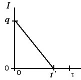
The results of the analysis
depend on the lot size and the service level. The figure
shows that the maximum inventory is the same as the order
level. In addition to the other results computed for the
no-shortages case we now can compute:
- Maximum inventory level: This is q.
- Minimum inventory level: This is 0.
- Service Level: This is v. The satisfied
demand in a cycle is Dt', where t' = v*(cycle
time).
|
|
The Inventory Model |
| |
|
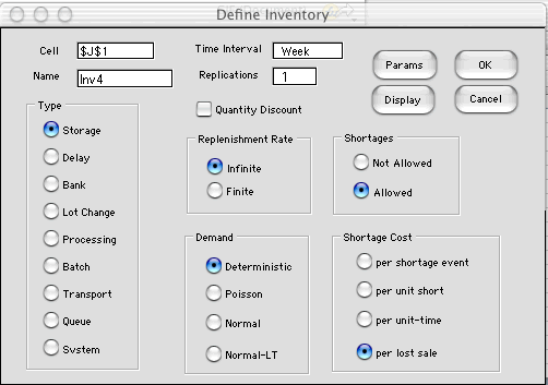
As before, we create a model
by selecting Add Inventory from the menu. We
select per lost sale from the Shortage Cost
options frame on the dialog.
|
| The lost sales case is interesting because
the optimum solution is to allow no shortages or to satisfy
none of the demand. The two cases are below for an example.
On the left, Ex4 A, when the unit cost of a lost sale is
$3, the optimum policy is the same as the policy when no
shortages are allowed. In the case at the right, Ex4 B,
when the lost sales cost is $2, the optimum policy has the
lot size and service level both at 0. The optimum cost is
the cost when all demand is lost. We have modified the example
for this illustration by setting the product revenues and
costs both to zero. The lost sales cost represents the net
revenue loss on a sale plus any additional penalties due
to the lost sale. |
|
Finite Replenishment
Rate and Backorders |
| |
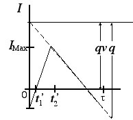
The figure
below illustrates this case. On-hand inventories are in blue
and backordered quantities are in red.
No new notation is required for this case. |
Single Cycle |
| |
|
At the start of the cycle,
the inventory grows at the rate P - D until the
lot size is produced and then declines at the rate D.
From time 0 to t1' the production is satisfying backorder
demand and current demand. From t1' to t2' production
adds to inventory. From t2' until the end of the cycle,
the inventory decreases at the demand rate D. |
|
The Inventory Model |
| |
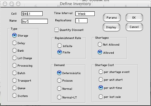 |
As before, we create a model
by selecting Add Inventory from the menu. We
select Finite from the Replenishment
options and per unit-time from the Shortage
Cost options on the dialog.
|
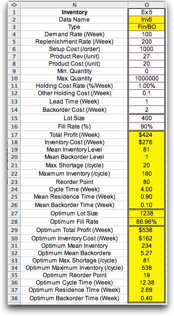 |
The results depend on both
the lot size and fill rate.
The optimum solution balances order cost, inventory cost
and backorder cost. |
|
Finite Replenishment
Rate and Lost Sales |
| |
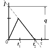
The figure
below illustrates this case. Inventories are blue. Since shortages
are lost there is no backorder region.
No new notation is required for this case. |
Single Cycle |
| |
|
At the start of the cycle,
the inventory grows at the rate P - D until the
lot size is produced and then declines at the rate D.
From time 0 to t1' the production is satisfying current
demand and building inventory. From t1' to t2' inventory
decreases until it reaches 0. From t2' until the end of
the cycle, the inventory remains at 0 while sales are lost. |
|
The Inventory Model |
| |
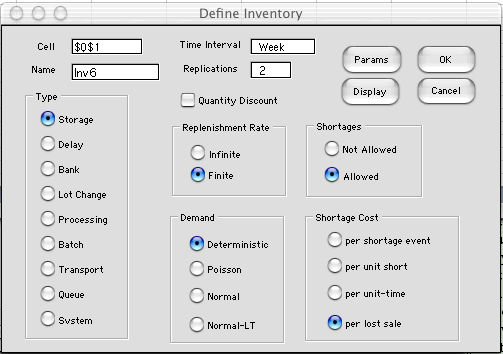 |
As before, we create a model
by selecting Add Inventory from the menu and
select the appropriate options
Again we see the result that the optimum either has no
shortages or satisfies none of the demand. With a shortage
cost of $2 per unit, the optimum policy is to allow no
shortages as shown on the left. With a cost of $1 per
unit, no inventory is maintained as shown on the right. |
|
| |
|
