| |
|
When several items are stored
in inventory, there may be restrictions on features of
the inventory system that involve all the items. For example,
all inventories involve investment, and it may be that
the total capital available for investment in inventories
is limited. In this case we want to maximize total profit
or minimize total inventory costs subject to a constraint
on total inventory investment. This is an optimization
problem. The add-in constructs models for three different
optimization problems that have been discussed in the
literature. All the models allow several different constraints
to be placed on the system.
Optimization models are defined by selecting the Optimize
command from the menu. |
The optimization problems considered include the
following.
- Multiple Item: This option refers to the situation in which
two or more items are stored in the inventory system and there
are constraints on the system.
- Common Cycle Time: For this option, the system is operated
so that replenishment orders are placed on a regular time
cycle. The several items in the inventory must all be replenished
with the same interval between replenishments or with integer
multiples of the system cycle time.
- Machine Scheduling: Here we consider several items produced
on the same machine. The items usually have finite production
rates and non-zero setup times. The machine is scheduled on
a regular cycle. In each cycle all or some of the items are
produced. The replenishment of a specific item occurs in each
cycle or in some multiple of the machine cycle time. In addition
to the system constraints allowed for the other models, a
constraint on total machine availability is introduced. A
variable is added to allow more than one machine to be used
for the system.
|
Warning
The add-in builds the optimization models using
the Math Programming add-in, so this add-in must be installed
for the optimization option. Models are solved with the
Excel Solver add-in. In order to use this add-in it must
be installed. In addition, before building a model, the
user must open the Solver dialog, reached from the Tools
menu. This establishes a link to the Solver add-in, and
this step must be done or the model building process will
not work.
The models constructed are nonlinear and in
some cases involve integer variables. Optimization
models involving nonlinear functions and integer variables
are hard to solve. After solving a problem once using
the Solve button on the worksheet, solve the problem
again several times using Solver directly. Experiment
with different Solver parameters such as: Precision,
Tolerance and Convergence. Use several starting values
for the solution variables and select the best of several
Solver solutions. |
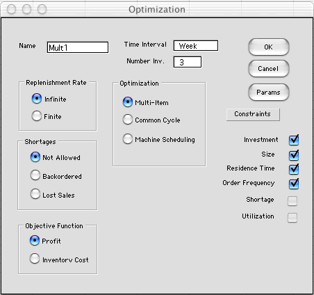
When the Optimize command is selected,
a dialog is presented that allows features of the system to
be described. The dialog is shown below.

By clicking the buttons on the left, the features
of the several inventories are specified. All items have the
same features. The optimization options only consider deterministic
systems. The Params button allows the user to specify
default parameters for the items. When first placed on the worksheet
all the items have the same parameters, but they may be changed
directly on the worksheet.
The buttons in the center, determine the kind
of optimization problem to be modeled. The boxes on the right
determine the constraints that will be included. At least one
constraint must be selected for a meaningful analysis. The Shortage
constraint is available only for those systems that allow
shortages. The Utilization constraint is available
for the Common Cycle problem. It is required for the
Machine Scheduling problem. We will explain the constraints
on the following pages that show specific examples of each type. |


