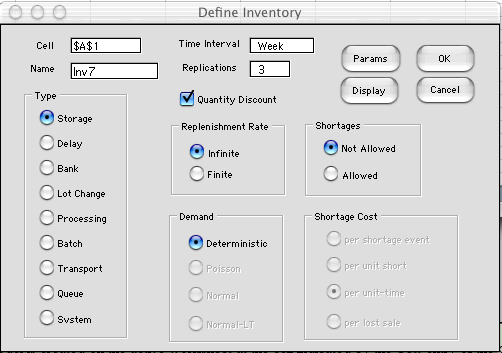
The price of a raw material for a production process may be reduced if a sufficiently large quantity is purchased at each inventory replenishment. A price reduction that occurs at some puchase level is called a quantity discount. A model that solves the quantity discount problem is constructed by clicking the Quantity Discount button on the dialog. The entry for number of replications near the top of the dialog specifies the number of different segments of cost. This number must be greater than 1. For the example we have chosen 3. We have chosen no instance results on the dialog, instead concentrating on the some of the optimum results.

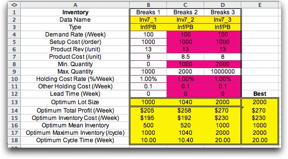
The model is created on the active worksheet at the cell indicated by the Cell entry of the dialog. Three inventory models are provided. The pink cells indicate equations that link the parameters to the first model, in column B. This makes it simpler to enter data for quantities that usually do not change over the options. The equations in the pink fields can be replaced by numbers if the situation does not have common inventory characteristics for all the cost segments.

Note that row 7 holding the product cost is not colored indicating that the different cost levels are to be entered in this row. Also in row 9 remains white. The maximum of the ranges of the cost levels are entered in this row. The maximum of one segment is automatically transferred to the minimum of the next higher segment.

Below the data, the optimum results for each cost level is presented. The optimum in each case is constrained by the lower and upper range for the associated cost.

To the right, in column E, the best alternative is selected. In this case it is optimum to purchase lots of 2000 units. Although the optimum policy for a cost of $8.50 is to purchase 1040 units in a lot, the profit for this option is less than the profit obtained by purchasing 2000 units at a cost of $8.00 each. The higher inventory cost at the greater lot size is offset by the lower unit cost.