| This
model is similar to the other models, but it represents a somewhat
different system. Here we have a single machine type producing
several products. The products correspond to the individual
items used for the other optimization models. For most instances
of this problem, the individual items have finite replenishment
rates, representing the production rates on the machine. The
products also have setup times, representing the time required
to setup the machine to produce the individual products. Although
we allow the constraints used by the other models, the principal
constraint for this situation is the machine utilization constraint.
If there is only one machine of this type, the total proportion
of the times spent in production or setup cannot exceed 1. In
our models we allow the number of machines to be variable, so
the constraint is changed so that the total utilization of the
machine type cannot exceed m where m is the
number of machines used.
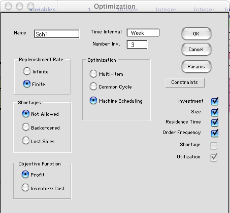
To create a model, we select Optimize from
the menu and click the Machine Scheduling button. The
model created is similar to the common cycle model. Note that
the Utilization constraint is required for this model.
The dialog does not allow it to be unchecked.

To illustrate, we use the same situation as for
the common cycle example, but here the replenishment rates
are finite. They represent the production rates of the three
products using the machine. Of course, the rates must be greater
than the demand rate for feasibility.
Reviewing the worksheet below, we note that the
first variable is System Cycle Time (Sys CT). This
is the cycle time for the machine. We have three variables for
the items, N1, N2 and N3, representing the relative cycle times
for the three products. The value of 1 means that the item is
produced in every cycle. The value of 2 means that the item
is produced every other cycle. Higher values have similar meanings.
The relative cycle times must be integer. For this model we
have one additional variable, Number of Resources.
This is the number of machines used for the system. For some
situations it may be impossible to meet the production requirements
with a single machine. This variable allows the solution to
use an integer number of machines, greater than 1.
The yellow cells in column H through K hold nonlinear
expressions of the decision variables that define the investment,
size, residence time, order frequency and utilization for the
system. The profit is a separable nonlinear function of the
decision variables.
The worksheet is shown below with the optimum
solution. The optimum solution uses 2 machines. The Solver could
find no feasible solution when the number of machines was limited
to 1. |


