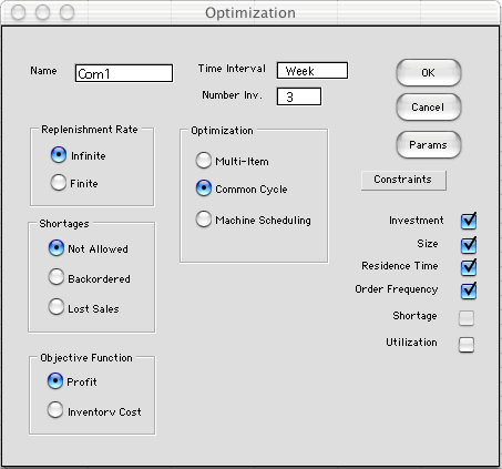
The common
cycle time problem is similar to the multi-item problem except
that here we restrict the cycle times of the items to either
be the same or be integral multiples of a common cycle time.
This kind of system would be used when it is more convenient
to order replenishments for several items at a time. Again we
select Optimize from the menu, but this time we select
the Common Cycle button. We do not repeat features
of the model that are same as the multi-item case.

For the example we use a similar inventory system
as we used to illustrate the multi-item case. For this system,
however, there is an setup cost to place an order for the entire
system. There may also be additional setup costs for each item.
Reviewing the worksheet below, note that in addition
to the three columns for the individual items, there is a fourth
column for the system. The only data included in this column
is the system setup cost.
The variables of the math-programming model for
the common cycle situation are quite different than the variables
for the multi-item system. The principal variable is System
Cycle Time (Sys CT), measured in weeks for the example.
The variables labeled N1, N2 and N3 are the relative order
cycles for the items. A value of 1 means that the item is
ordered in every cycle of the system. A value of 2 means
that the item is ordered every other cycle. These variables
are restricted to integer values. The default upper and
lower bounds for the integer variables are both 1, meaning
that every item is ordered in every cycle. We have changed
the upper bound to 10 to allow variability above 1. The
worksheet is shown below with the optimum solution.
The yellow cells in column H through K hold nonlinear
expressions of the decision variables that define the investment,
size, residence time and order frequency for the system. The
profit is a separable nonlinear function of the decision variables. |


