The line is a series of operations that all carry the same flow. For the push line, the flow is enters the first operation and passes through the line to the last one. We show as an example a line with five operations with flow pushed from the first.

The Excel worksheet for a numerical example is shown below. Note that the titles in the display are more general than for individual operations since the columns of the system display represent different kinds of operations. Row 1 holds the operation names provided by the modeler. Row 2 holds the name used for named ranges created by the computer. These entries should not be changed. Row 3 defines the types of operation. The types available are the WIP component types described previously. The program uses the first 3 letters to identify the type.

Rows 5 through 11 hold data describing the individual operations. We have created a hypothetical situation for our example.

The push line has all flows determined by the flow rate entry for operation A, cell B4. This cell has a white background indicating that it is under the control of the modeler. The cells to the right in row 4 are colored yellow to indicate that they are determined by formulas. The flow formula makes the cell value equal to the value of the cell on the left.

Operation A represents the raw material ordering process where the lot size is 10 units. The material passes through process B with nonzero setup time and unit processing time. To reduce the effect of the setup time we produce lots of 5 units. We then pass to the transportation operation, C. The setup time in this case is the fixed time to move 10 items. We move lots of size 10, but then separate the lots into individual items.

Operation D is a process with a queue. Although we are assuming a constant flow rate, the queuing models assume variability in the arrival and service activities. Operation D processes lots of 2 and then sends individual items into operation E. Operation E is the finished goods inventory. The policy is to have an average of 25 units in this inventory, represented as a bank. The bank operation, E, has data items indicated by x. The numbers in these cells do not affect the results.

Row 5 holds the unit values. For a line system, the values increase as the product passes through the line. The difference between the value at an operation and the value at its predecessor is the value added by the operation.

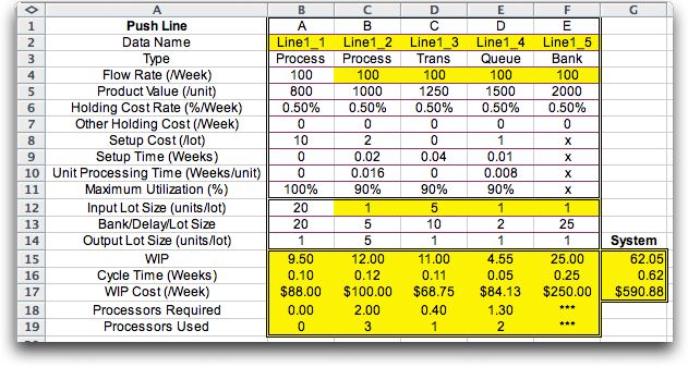
Rows 12 through 14 hold the variables for the operations. In all cases, the first variable, row 12, is the input lot size and the third variable, row 14, is the output lot size. We assume that lot sizes can only change at an operation. The program has placed formulas in row 12 so that the input lot sizes for operations B through E are equal to the output lot size of the previous operations. The input lot size of the first operation, the process lot sizes and the output lot sizes are under control of modeler.

For operations that involve processing, the second instance variable is the process lot size. For the bank operation, the second instance variable in row 13 is bank size rather than lot size. For a delay, the second variable is the time of delay. For a lot size change operation, the second variable is ignored.

The analysis appears in rows 15 and following. The WIP is computed for each operation in row 15. The cycle times computed with Little's Law are in row 16. The costs of holding WIP and for setups is in row 17. For processing, batch and queuing operations we compute the number of machine processors required to meet the specified flow rate. These numbers are reported as fractions in row 18 because more than one operation may require the same processor and fractional numbers represent partial use. Given the maximum utilization data from row 11, we compute the integer number of machines required. These numbers are reported in row 19. For the queuing station, the number in row 19 is the number of servers.

The system results are totaled in column G. For a line, the cycle time is simply the sum of the cycle times of the operations. This is not generally true for the other structure options.

We have observed three factors that link the operations of the system, flow, lot size and unit value. For the line system, formulas provide the appropriate links for flow and lot size. Insertion of the correct unit values is the responsibility of the modeler.

Pull Line

Using the same example, we see below that the pull option gives the same result as the push option for the line. The difference is that in the pull system, flow is pulled out of the system from the output of operation E, as indicated by the white color of the flow rate for operation E. The flows through the other operations are equal to the flows through the subsequent operations. Also observe that the lot size relations are different for a pull line. The output lot size of an operation is set equal to the input lot size of the following operation.