|
|
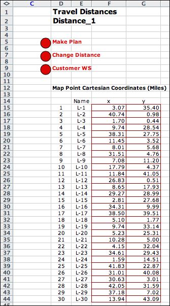
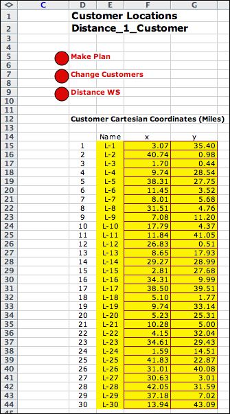
This page investigates the various
options for problem complexity. The examples of this page are
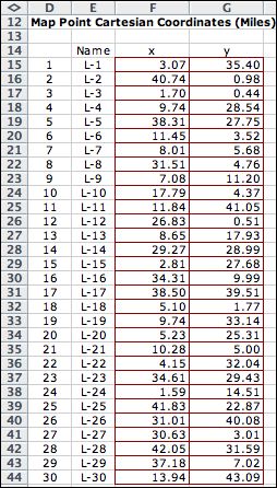
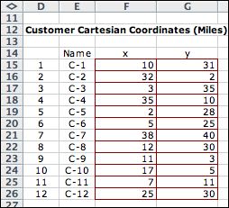
on the routing_demo.xls file. The figure below shows
the distance and customer
lists for all the examples except the last one. We keep the
problems small to more easily show the features of the worksheets
created by the add-in. In this case the customer and distance
locations are the same. The last example on this page shows
a case where they are different.
|
TSP Considering only Distance |
| |
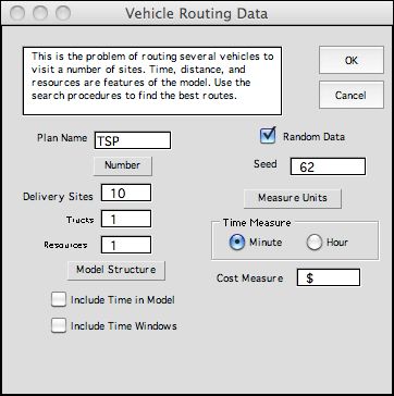
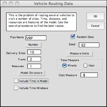
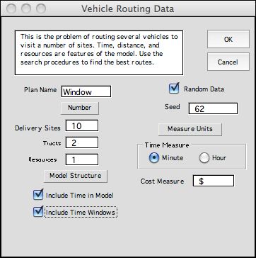
Plans are constructed by clicking
the Make Plan button on either the distance or the data
sheet. The dialog shown below accepts a name for the plan, TSP
for the example. Fields are provided to specify the number of
deliveries, trucks and resources. When clicked the Random
Data checkbox calls a random number generator to choose
the parameters of the problem. The seed controls the sequence
of random numbers generated.
The two checkboxes at the bottom specify the
structure of the model. Leaving both options unchecked, we build
a model that does not include time or time windows. |
| |
|
| |
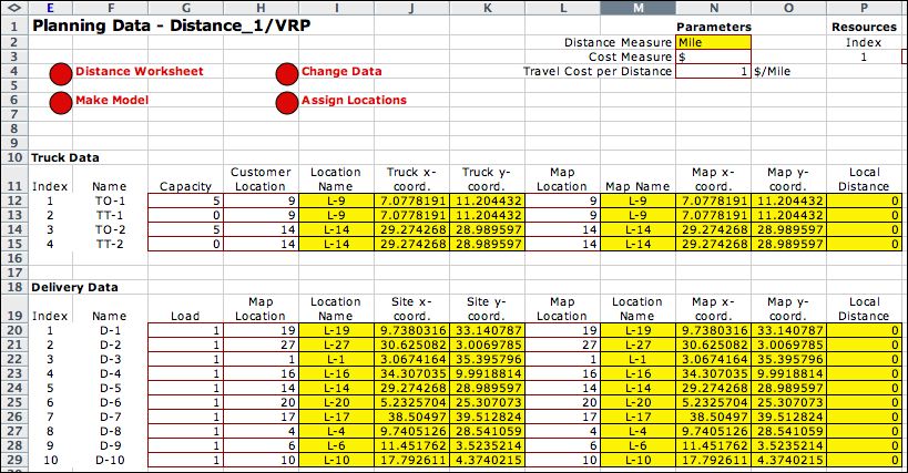
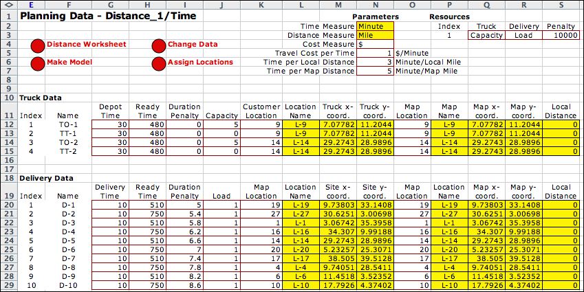
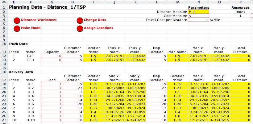
Clicking OK builds the planning
data worksheet shown below. Column H holds indices to the customer
list. The truck is represented by two entries, one for the
origin location of the truck and one for the terminal location.
Here we assign customer location 9 to both. The location name
and coordinates are passed to this worksheet from the customer
worksheet via Excel formulas.
The map locations are assigned in column L. In general, these
may be different than the customer locations, but when the
distance and customer worksheets have the same location lists,
a customer is assigned to the same map index
as customer index. The location name and coordinates are transferred
by equations from the distance worksheet. The local distance
in column P is the distance from the customer location to the
map location. Since the example has these co-located, the local
distance is zero.
The only resource used for the example is truck capacity.
The numbers in column G give the capacity values for the trucks
and the loads for the deliveries. Loads subtract from the capacity,
so this constraint is not affective for the TSP example. |
|
| |
We more formally list the columns
of the planning
data worksheet below. The TSP model is the simplest type, additional
columns are added for the time and time window options.
| Name |
The default names are assigned as in the example, but can
be changed to identify specific vehicles and delivery points.
Two entries are required for each truck representing its
starting location, TO-1, and its terminal location, TT-1. The
letter O stands for origin, and the letter T stands
for terminal. Each truck occupies two rows of the
table, even numbered rows are out-going and odd numbered
rows and in-coming. |
| Capacity/Load |
The first resource constraint is automatically named the
capacity. The loads associated with the delivery sites use
the capacity of a truck. The default load for each site is
1 and the default capacity of each truck is the total load
divided by the number of trips rounded to the next integer.
Capacities may reflect any limitation on trucks and multiple
resources may be defined. Each will receive a column for
data on the plan. There is a penalty for violating the capacity
constraint. The penalty is charged for each unit of capacity
in excess of the amount available. The capacity constraint
for the example, will assure an equal number of delivery
sites for each truck if the penalty is set high enough. |
| Customer Location |
This is the index of the table on the customer worksheet
that identifies the location of the truck or delivery. |
| Customer Location Name |
The names are transferred from the customer worksheet. |
| Customer Geometric or Cartesian Coordinates |
There are two columns that express the coordinates of the
customer locations specified as latitude and longitude for
geometric coordinates and x and y for Cartesian coordinates.
The cells are yellow because formulas in these columns link
to the map location information on the customer worksheet. |
| Map Location |
This is the index of the table on the distance worksheet
that identifies the map location of the truck or delivery.
The map location is assigned as the closest map location
to the delivery site or truck depot. |
| Map Location Name |
The names are transferred from the distance worksheet. |
Map Geometric or Cartesian Coordinates |
There are two columns that express the coordinates of the
customer locations specified as latitude and longitude for
geometric coordinates and x and y for Cartesian coordinates.
The cells are yellow because formulas in these columns link
to the map location information on the customer worksheet. |
| Local Distance |
This is the Euclidean distance between the assigned map
coordinates and the truck or delivery site coordinates. When
travel takes place from one site to another, the trip is
assumed to be the map distance between the two sites plus
the sum of the two local distances. Both local distance and
the distance between map locations are assessed costs that
are proportional to the cost per unit time and travel time
per unit distance. |
|
| |
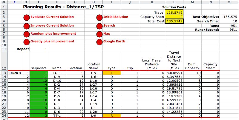
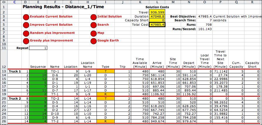
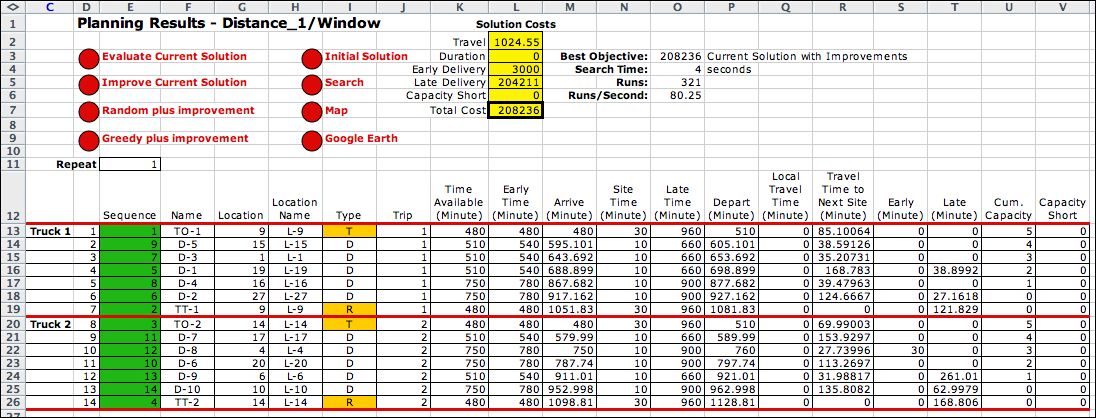
The Results worksheet for
the example is below. This worksheet shows a solution to the
TSP. The solution is given in column E as the sequence of truck
and
delivery
map locations that will be followed by the single truck. The
solution process starts with an initial sequence that starts
at the truck origin location, visits the delivery sites in numerical
order and finishes at the truck terminal location. The solution
is modified by various heuristics until a local optimum solution
is obtained. That solution is reported below. All the examples
on this page follow the same process, so the results are comparable. |
|
VRP Considering only Distance |
| |
The second example uses two trucks
for the deliveries. We call this the vehicle routing
problem (VRP). Each truck has the
resource capacities of
5, so the solution should have two tours of five deliveries.
The only change in the dialog from the TSP example is the number
of trucks. |
| |
|
| |
Each truck has two rows and each
delivery has one. For this example we assign the trucks to two
different locations, L-9 and L-14. |
|
| |
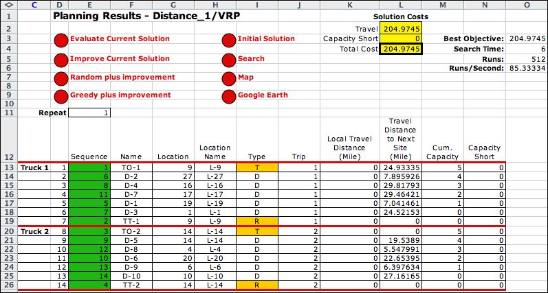
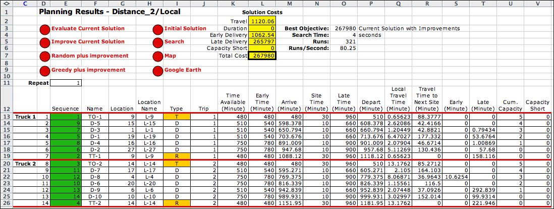
The results after improvement show
two routes,
one for each truck. The total cost, about 205, is larger than
the cost for the TSP, about 136. |
|
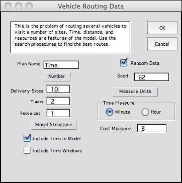
VRP Considering Distance and Time |
| |
Click the Include Time button on
the dialog for the new model. |
|
| |
The planning data worksheet for
this case is shown below. Columns are added to hold the time
data for the trucks and deliveries. Also new parameters transform
distances to times. |
|
| |
The table defines the columns
holding the time data.
| Depot Time or Delivery Time |
This is the fixed time to load a truck or make a delivery.
The time that a truck leaves the site is the arrival time
plus the delivery (depot) time. |
| Ready Time |
This is the earliest time that a particular truck may
start or that a particular site will accept a delivery.
This is a hard constraint. If a truck reaches a site before
the ready time, it must wait to begin the delivery process.
For the origin node of a truck, the time will indicate
the time the truck begins its route. |
| Early Time |
This is a scheduled earliest time for a truck to arrive
at a delivery site. The truck may arrive before this time,
but a penalty will be assessed. The early time differs
from the ready time in that the early time constraint may
be violated, but at a penalty, while the ready time constraint
is never violated by a solution. |
| Late Time |
This is a scheduled latest time for a truck to leave
a delivery site. The truck may leave after this time, but
a penalty will be assessed. A truck leaves a site at the
arrival time plus the delivery (or depot) time. For the
terminal site of a truck, this might be the end of the
working day. |
| Duration Penalty |
When a truck leaves a site, the solution is assessed
a cost that is the duration penalty multiplied by the leaving
time. This parameter can reflect priorities with sites
having greater duration penalties having higher priorities. |
|
| |
The solution to the example is
below. For this model the cost model depends on time. The travel
cost component
is the total distance divided by the velocity and multiplied
by the cost
per minute. The solution mirrors the dual effects of distance
and duration penalties. |
|
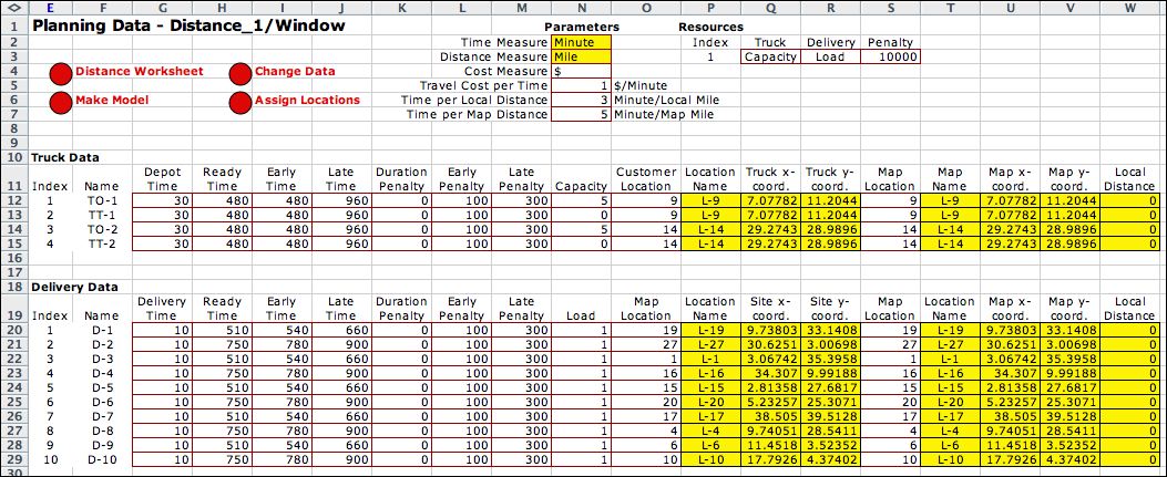
VRP Considering Distance, Time and Time Windows |
| |
Time windows express customer requirements
for early and late delivery. For the time window feature
click the Include Time Windows checkbox. |
|
| |
The data worksheet with time windows
is below. |
|
| |
New columns in the data determine
the time windows and the penalties for violating the time windows.
| Early Time |
This is a scheduled earliest time for a truck to arrive
at a delivery site. The truck may arrive before this time,
but a penalty will be assessed. The early time differs
from the ready time in that the early time constraint may
be violated, but at a penalty, while the ready time constraint
is never violated by a solution. |
| Late Time |
This is a scheduled latest time for a truck to leave
a delivery site. The truck may leave after this time, but
a penalty will be assessed. A truck leaves a site at the
arrival time plus the delivery (or depot) time. For the
terminal site of a truck, this might be the end of the
working day. |
| Early Penalty |
When a truck arrives at a site before the early time,
the solution is assessed a cost that is the early penalty
multiplied by the difference between the early time and
the arrival time. When a truck arrives after the early
time, no early penalty is charged. |
| Late Penalty |
When a truck leaves a site after the late time, the solution
is assessed a cost that is the late penalty multiplied
by the difference between the leaving time and the late
time. When a truck leaves before the late time, no late
penalty is charged. |
For simplicity we have made the duration penalties 0 for this
example. |
| |
The solution for this model tries
to meet the time windows. For the example this is impossible.
D-8 is visited early (Column S) and several deliveries are late (Column
T). Time windows for trucks model the desired leaving and returning
tins for the trucks. Both trucks return to their depots late. |
|
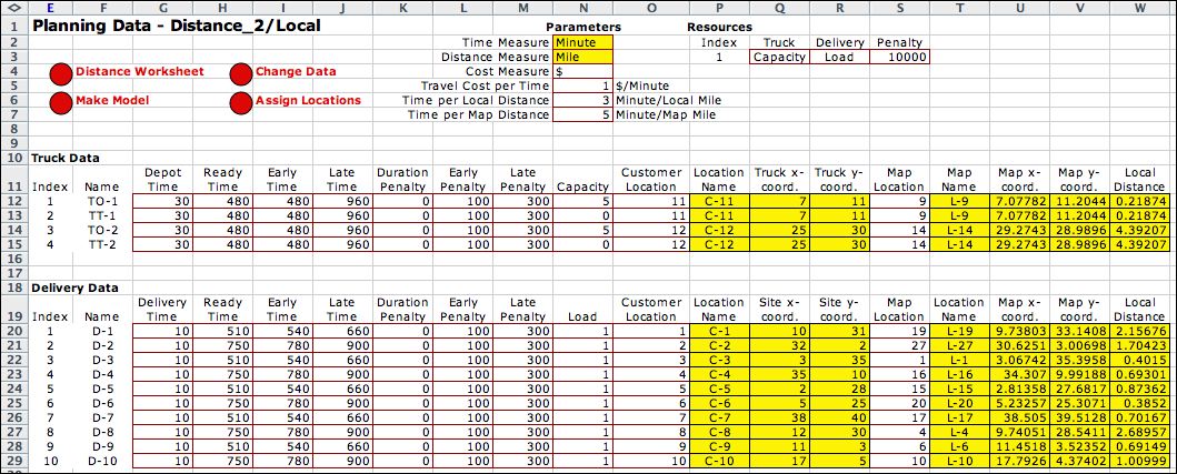
Nonzero Local Distances. |
| |
Nonzero local distances occur
when the locations on the distance worksheet are different
than the distances on the customer worksheet. The example uses
the data below.
|
| |
The example uses the data from
the previous examples, but specifies different customer and
map locations. The local distances are computed in column W.
| Local Distance |
With Cartesian coordinates this column holds the Euclidean
distances between the assigned map coordinates and the
truck or delivery site coordinates. For geometric coordinates,
the Great Circle distance is the metric. When travel takes
place from one site to another, the trip is assumed to
be the map distance between the two sites plus the sum
of the two local distances. Both local distance and the
distance between map locations are assessed costs that
are proportional to the cost per unit time and travel time
per unit distance. |
|
|
| |
When time is not included in the
model, such as the TSP in the first example, nonzero local distances
do not matter. When time is included, the local times are added
to the map travel times to find the total travel times between
two sites. This increases the time consumed by all parts of the
routes. Greater
total duration costs and time window costs are to be expected. |
|
Maps |
| |
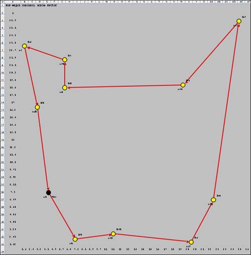
It is interesting to compare the
maps of the five cases considered above. The TSP has a single
route
where all others have two. Yellow dots show delivery locations
and black dots show truck locations. In the green route
for the VRP map, one of the deliveries has the same location
as the truck. The yellow dots take preference. |
TSP Map
 |
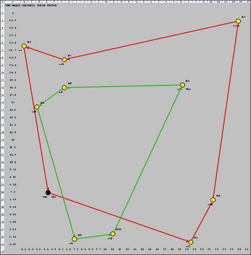
VRP Map
 |
VRP with Time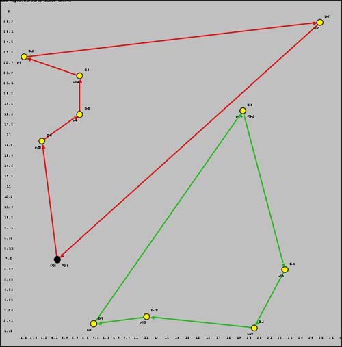
|
VRP with Time and Windows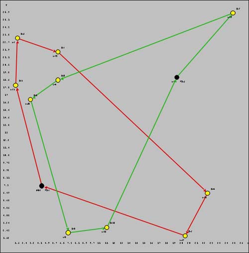
|
VRP with nonzero Local Distances
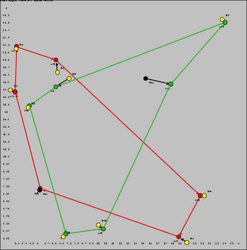 |
For the last example, local distances are nonzero. The
local distances are shown with black lines outside the routes.
The black and yellow dots are not directly on the routes
but connect to red or green dots on the route. The red and
green dots are map locations. |
|
| |
We provide these examples to illustrate
the options available for problem definition. We return to these
examples to discuss solution procedures. |
| |
|