|
|
 |
Vehicle
Routing |
 |
-
Planning Data |
|
|
The Planning Data worksheet
holds data specific to a particular routing problem. Clicking
the Make Plan button at the top of the Distance worksheet
for the Austin example creates the worksheet. The Vehicle
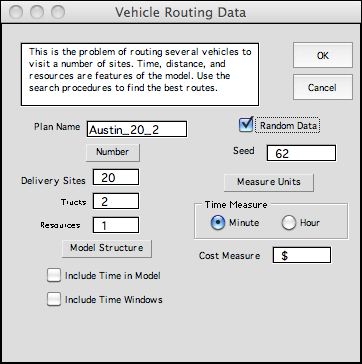
Routing Data dialog
accepts data for a plan. A Distance worksheet may
have several plans, but each Planning Data worksheet
is based on a specific Distance worksheet.
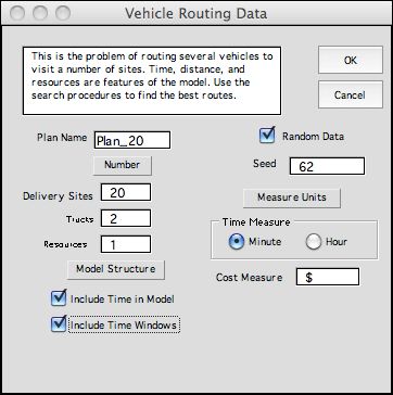
A plan has a name that is used to name the worksheet created
at this step. Many named ranges on the worksheet also use the
name. The name may contain only alphanumeric characters with
no spaces or punctuation. It cannot be changed once the worksheet
is created. Do not change the name on the worksheet tab. Three
numeric fields define a plan: the number of deliveries, the
number of trucks, and the number of resources. The Random
Data checkbox causes the add-in to insert random data
into some of the data fields. The Seed controls the
random number stream. The time measure is specified as hours
or minutes. The cost measure is the field on the lower right.
Here is the symbol for U.S. dollars ($).
The dialog accepts the number of deliveries to be made and
the number of individual vehicles (called trucks)
used to make the deliveries. A truck begins its route at
some starting point, visits a collection of delivery sites,
and completes its route at a finish point. The start
and finish points are usually at the same place for a given
truck, but the data can specify different places. Different
trucks will serve their routes simultaneously.
Deliveries use truck resources such as space or weight.
Our example uses a single resource called capacity. Each
delivery requires one unit of capacity (capacity utilized is
called load) and the default value of the truck
capacity is the number of deliveries divided by the number
of trucks rounded up to the nearest integer. For example, two
trucks making 20 deliveries will each have a capacity of 10.
A constraint of this kind partitions the deliveries into trips
with a different truck for each trip. |
Example |
| |
An example plan is shown below. We
discuss the various data items below the figure. Click the picture
to open a window with a larger image. |
|
| |
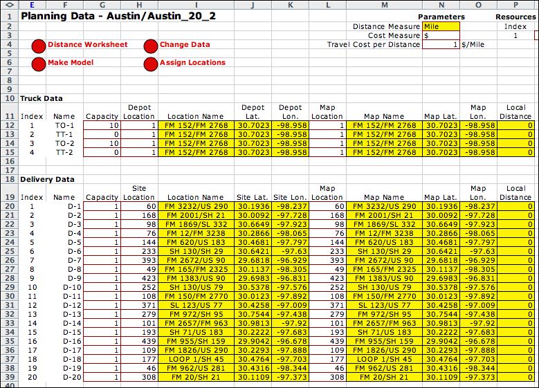
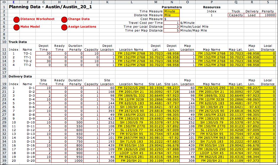
The data has three parts: the
parameters at the top, the truck data starting in
row 11, and the delivery data staring in row 19. The parameters
in column N define three constants related to time, distance
and cost in N2, N3 and N4. The next entry, N5, requires an
estimate of cost per unit of travel time. The principal mode
of travel for vehicles is on the routes between map locations,
however, truck depots and delivery sites may be located at
geographic locations not on the map. Travel between two
sites on a route has three parts, travel from the local location
of the first site to a nearby map location, travel from one
map location to a another, and finally travel to the local
location for the truck. Entries in cells N6 and N7 specify
the travel time per unit distance for local and map travel.
For the example, we assume the cost measure is dollars
and the time measure is minutes, so the example shows $1
per minute in N5. The entry in N6 is the time required for
distances traveled between locations on the Distance worksheet.
If we measure time in minutes, the example specifies 3 minutes
per mile (20 miles an hour) for travel between map locations.
N7 shows the time required for each unit of distance traveled
from a map location to the site of a delivery. We call this
the local distance. The example shows 5 minutes per mile or
12 miles an hour. This assumes travel between locations defined
by the Distance worksheet
is faster than local travel.
The resource data starting in column Q gives the names for
the resources when applied to trucks, Q3, the names for deliveries,
R3, and the penalties for using more resource than is available,
S3. When a single resource is specified, the default names
are capacity and load.
The penalty value, 1000, for the example, is used by the
optimization to penalize violations of the resource constraint.
One might increase or decrease this number depending on the
flexibility of the resource.
The truck and delivery data have similar columns. All the
data in these columns may be set by the user except the yellow
fields. The customer location column is column O. These entries
are the indices from the customer worksheet. For the example
we assign the start and finish locations for the trucks as
customer location 1. If we look on the customer worksheet we
find this site has the name FM 152/FM 2023, indicating the
intersection of two farm roads. The geographic coordinates
of this location are transferred from the customer worksheet
by formulas using the entry in column O as the index. In a
similar fashion the locations of the deliveries are specified
by indices to entries on the customer worksheet. For the example,
these numbers were assigned randomly. For an actual case they
would be determined by the delivery schedule for the day.
The entries in column S are indices of the table on the distance
worksheet. These define the name, latitude and longitude to
the map location assigned to the truck or delivery. We assign
a map location to as close as possible to the customer location.
For the Austin example, the customer list is the same as the
map table, so the map location assignment is the same as the
customer location. In general, customer locations will not
be the same as map locations. To find the closest map points
to the customer locations click the Assign Locations button
at the top of the worksheet. This button evaluates sequentially
assigns each customer location to the test point cells
on the distance worksheet. The minimum distance point in column
K of the customer worksheet is placed in column S.
The distance between a customer location and the assigned
map location is called the Local
Distance.
This field is computed with Excel formulas. Since the customer
and map worksheets are the same for the example, the local
distances are all zero. |
| |
The several columns of the plan
worksheet are listed below. To keep the example simple, the
example uses the default values of the parameters except the
location indices.
| Name |
The default names are assigned as in the example,
but can be changed to identify specific vehicles and delivery
points. Two entries are required for each truck representing
its starting location, TO-1, and its terminal location, TT-1. The
letter O stands for origin, and the letter T stands
for terminal. Each truck occupies two rows of the
table, even numbered rows are out-going and odd numbered
rows and in-coming. |
| Depot Time or Delivery Time |
This is the fixed time to load a truck or make a delivery.
The time that a truck leaves the site is the arrival time
plus the delivery (depot) time. |
| Ready Time |
This is the earliest time that a particular truck may start
or that a particular site will accept a delivery. This is
a hard constraint. If a truck reaches a site before the ready
time, it must wait to begin the delivery process. For the
origin node of a truck, the time will indicate the time
the truck begins its route. |
| Early Time |
This is a scheduled earliest time for a truck to arrive
at a delivery site. The truck may arrive before this time,
but a penalty will be assessed. The early time differs from
the ready time in that the early time constraint may be violated,
but at a penalty, while the ready time constraint is never
violated by a solution. |
| Late Time |
This is a scheduled latest time for a truck to leave a
delivery site. The truck may leave after this time, but a
penalty will be assessed. A truck leaves a site at the arrival
time plus the delivery (or depot) time. For the terminal
site of a truck, this might be the end of the working day. |
| Duration Penalty |
When a truck leaves a site, the solution is assessed a
cost that is the duration penalty multiplied by the leaving
time. This parameter can reflect priorities with sites having
greater duration penalties having higher priorities. |
| Early Penalty |
When a truck arrives at a site before the early time, the
solution is assessed a cost that is the early penalty
multiplied by the difference between the early time and the
arrival time. When a truck arrives after the early time,
no early penalty is charged. |
| Late Penalty |
When a truck leaves a site after the late time, the
solution is assessed a cost that is the late penalty multiplied
by the difference between the leaving time and the late
time. When a truck leaves before the late time, no late penalty
is charged. |
| Capacity/Load |
The first resource constraint is automatically named the
capacity. The loads associated with the delivery sites use
the capacity of a truck. The default load for each site is
1 and the default capacity of each truck is the total load
divided by the number of trips rounded to the next integer.
Capacities may reflect any limitation on trucks
and multiple resources may be defined. Each will receive
a column for data on the plan. There is a penalty for violating
the capacity constraint. The penalty is charged for each
unit of capacity in excess of the amount available. The capacity
constraint for the example, will assure an equal number
of delivery sites for each truck if the penalty is set high
enough. |
| Customer Location |
This is the index of the table on the customer worksheet
that identifies the location of the truck or delivery. |
| Customer Location Name |
The names are transferred from the customer worksheet. |
| Customer Geometric or Cartesian Coordinates |
There are two columns that express the coordinates
of the customer locations specified as latitude and longitude
for geometric coordinates and x and y for Cartesian coordinates.
The cells are yellow because formulas in these columns link
to the map location information on the customer worksheet. |
| Map Location |
This is the index of the table on the distance worksheet
that identifies the map location of the truck or delivery.
The map location is assigned as the closest map location
to the delivery site or truck depot. |
| Map Location Name |
The names are transferred from the distance worksheet. |
Map Geometric or Cartesian Coordinates |
There are two columns that express the coordinates of the
customer locations specified as latitude and longitude for
geometric coordinates and x and y for Cartesian coordinates.
The cells are yellow because formulas in these columns link
to the map location information on the customer worksheet. |
| Local Distance |
This is the Euclidean distance between the assigned map
coordinates and the truck or delivery site coordinates. When
travel takes place from one site to another, the trip is
assumed to be the map distance between the
two sites plus the sum of the two local distances. Both local
distance and the distance between map locations are assessed
costs that are proportional to the cost per unit time and
travel time per unit distance. |
|
| |
The information entered on the Data worksheet
defines the set of the deliveries required for some interval
of time, perhaps a day of operation. The add-in tries to develop
a schedule that will meet the delivery requirements with the
trucks provided. The criterion is a composite cost
that includes the cost for travel, the total duration penalties,
the total early and late penalties, and the total resource violation
penalties. The model involves both time and distance as will
be reflected on the model worksheet.
We have entered sample data to the data worksheet. It represents
a problem with two trucks and twenty deliveries. Default values
are used for the time aspects of the problem. |
Alternative Data Forms |
| |
|
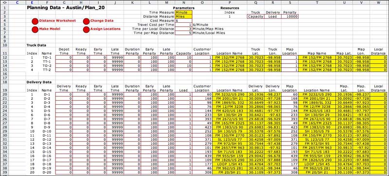
Although the example has columns for
time parameters, they did not effect to the solution.
The time delays for loading and unloading trucks are
all set to zero, so the time features of the model are
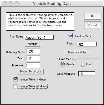
not effective. Options on the data dialog allow models
to exclude time and exclude time windows. The dialog
shows how to make a model that does not include
time. The checkbox for Include
Time in Model is simply left unchecked.
The planning data worksheet shown below is simplified
with the columns holding time data left out. The results
and model worksheets are similarly simplified. Note that
the cost only depends on the travel cost per mile. When
time is included the objective is to minimize the total
cost depends on the travel distance through the time
per travel mile and the cost per travel time parameters. |
|
|
| |
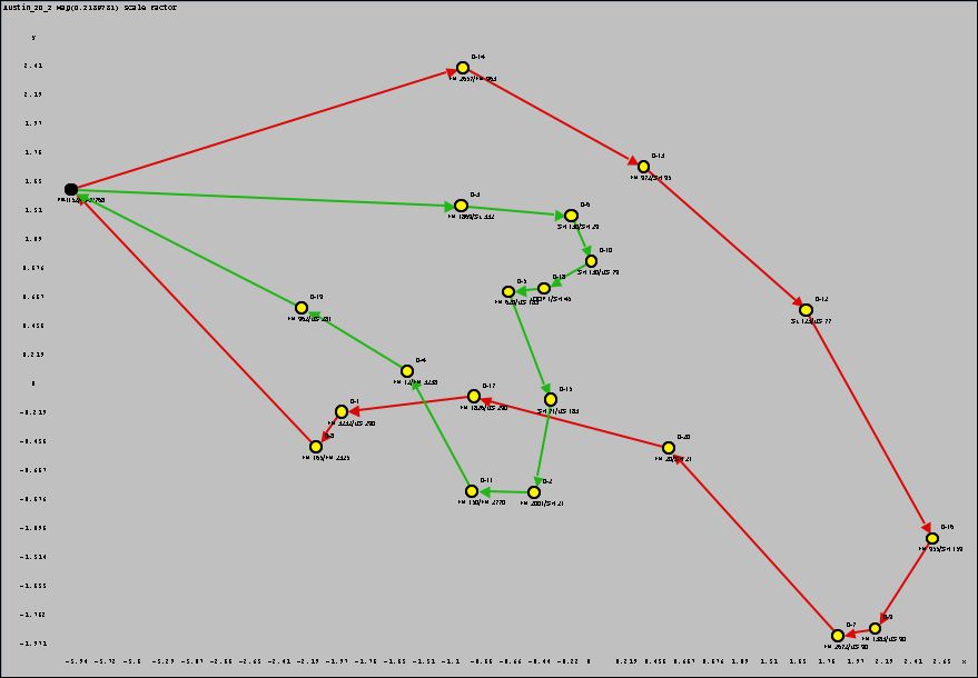
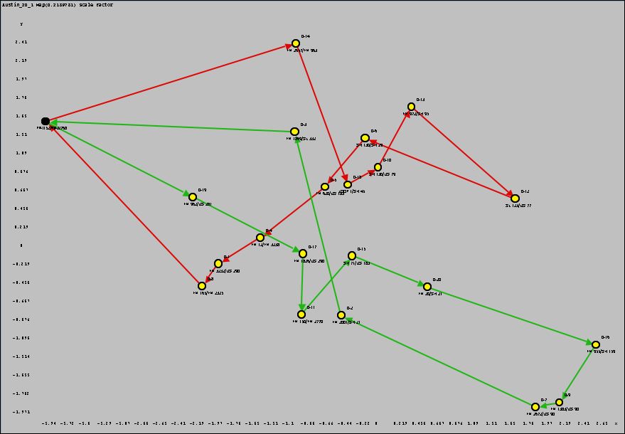
The map of the solution of the model
with no time features is below. This solution has the goal of
minimizing total distance where the two routes divide the deliveries.
The solution may not be optimum because heuristic solution methods
are used. |
|
| |
|
If the model is to represent time
but not time windows, leave the Include Time Windows box
unchecked. The plan in This case is shown below. We have
entered nonzero parameters for depot and site times. The
solution depends on the finish
time for each customer. On the data form we provide nonzero
penalties for the ten customers with the greatest indices. |
|
|
| |
The solution map shows the effect
of penalties. The solution has all the sites with nonzero penalties
visited first. |
| |
|
Changes |
| |
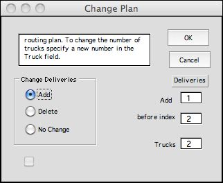
Once constructed, the number of
deliveries and the number of trucks
may be changed using the Change button.
The dialog below specifies the number of deliveries to be added
or deleted and the location of the change. To change the number
of trucks, specify a new value in the associated field. The
example adds a new delivery to the plan and places it above
the delivery that is currently second. The deliveries will
be re-indexed after the addition. New deliveries can't be added
before index 1. The last delivery cannot be deleted.
|
Buttons |
| |
At the top of the page there are
several buttons.
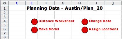
The Distance Worksheet button makes
the distance worksheet active. Each plan has a unique associated
distance worksheet. The Change Data button allows
changes in the plan. All features of the model can be changed
except the number of resources. The Assign Locations button
determines the closest map location to each delivery or depot
location. This is useful when the plan is given coordinates
for each truck and delivery site that are different than the
map locations. The Make Model button constructs the model and results worksheets
discussed on the following pages.
Data on the model worksheet are
directly linked to the contents of the planning data worksheet.
There is no need to create a new model when the data is changed,
however, if the numbers of trucks or deliveries change, a new
model is required. |
| |
|
|