|
|
 |
Vehicle
Routing |
 |
-
Results |
|
|
The Make Plan button
at the top of the Data worksheet creates two worksheets,
the Model worksheet and the Results worksheet.
The Model worksheet implements our model of the vehicle
routing problem. It is used by the Optimize Sequence add-in
to evaluate and improve solutions. The Results worksheet
reports the results of the solution algorithms. For the casual
user, it is not really necessary to learn all the details of
the model worksheet, so we present the results worksheet first.
Most of the figures on this page are reduced for presentation.
A larger version shows when the picture is clicked. |
Results Worksheet |
| |
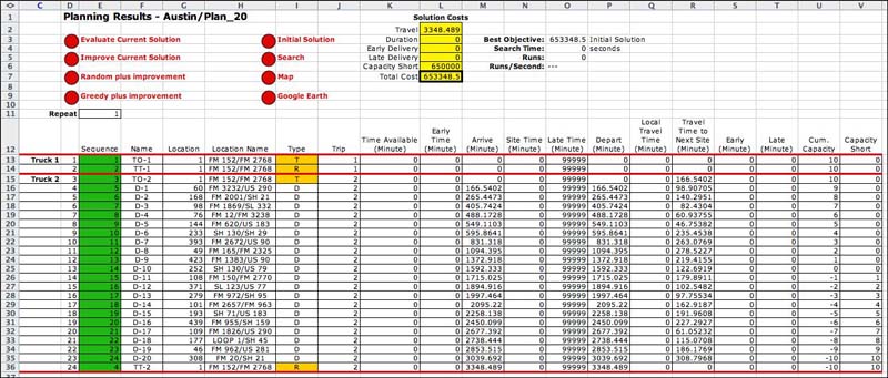
The figure below shows the results worksheet
as it first appears and before any attempt to find a good solution.
Click the figure to open a window with a larger illustration.
The solution is described by the sequence shown in column E.
The origin and terminal truck sites and the delivery sites
are each assigned a unique index with the trucks numbered first
and then the delivery sites. For the example, the first truck's
origin and terminal sites are numbered 1 and 2. The second
truck has sites numbered 3 and 4. The twenty deliveries are
indexed 5 through 24. The initial sequence is in index order
with one exception. The first three truck sites are first in
the sequence, followed by the delivery sites, and finally site
4, the terminal site of the last truck. This means that the
initial solution has all the deliveries assigned to the last
truck. Although this is not often a good solution, it is used
as a starting solution for the heuristic search methods to
be described later.
The Sequence column is shown in green to indicate
that the user may change the sequence. When one of the search
routines in invoked, the add-in fills this column with the
solution obtained. |
|
| |
Some of the columns of this form are taken
from the data worksheet and others are transferred from the
model worksheet. We list below the meanings of the
various columns. The contents of the columns are controlled
by the add-in so any user changes, except in the sequence column,
are neglected. The yellow cells at the top of the page hold
Excel formulas that hold the various cost components as computed
on the model worksheet. Our goal is to find a sequence that
minimizes the Total
Cost computed
in cell L7.
Red lines on the table indicate the start and finish of truck
routes.
For the initial solution the first truck begins at time 0,
visits no delivery sites, and immediate returns to its finish
site. The second truck then handles all the remaining deliveries.
Of course this not a good solution, but it will serve to illustrate
the columns of the form. |
| |
| Column C |
This is the untitled column C on the figure.
The column identifies where each truck begins its trip. |
| Column D |
This column is also untitled. It holds the indices of
the display |
| Sequence (E) |
The sequence is given by the indices assigned to the truck
and delivery sites. The initial sequence is in column E.
The solution sequence determined by the add-in will
be placed here. |
| Name (F) |
The names are assigned on the plan-data worksheet. |
| Location (G) |
The map locations are assigned on the plan-data worksheet. |
| Location Name (H) |
The map location names associated with the locations of
the truck and delivery sites. |
| Type (I) |
T indicates a truck origin and its terminal site
is R. Deliveries have the type D. |
| Trip (J) |
Trips are numbered sequentially. Truck 1 is always assigned
trip 1, but the trip numbers of other trucks and deliveries
depend on the sequence. |
| Time Available (K) |
This is assigned on the plan-data sheet. The default value
is 0. |
| Early Time (L) |
This is assigned on the plan-data sheet. The default value
is 0. |
| Arrive (M) |
This is the arrival time at a site. The arrival time is
computed considering the distances between adjacent sites
on the route, the delivery times and the available times.
Trucks run routes independently. A truck begins its trip
at the truck's available time, 0 for the example. The arrival
times for subsequent deliveries are determined on the model
worksheet. |
| Site Time (N) |
These times are defined on the plan-data sheet. |
| Late Time (O) |
This is assigned on the plan-data sheet. The default value
is 9999. |
| Depart (P) |
A truck departs from the site at the arrival time plus
the site time. The departure times are multiplied by the
duration penalties to compute the cost component of L3. |
| Local Travel Time (Q) |
After a truck departs a site, it must travel to the assigned
map location. The time for this trip is in this column. |
| Travel Time to Next Site (R) |
On leaving the customer location the truck travels the
local distance to the map point nearest the customer location.
The truck then travels to the map location of the next site
in the sequence. It then travels for the local time to reach
next customer location. Each of these distances are divided
by the velocity of the truck. This column shows the total
of these three times. |
| Early (S) |
This is the amount of violation of the early time constraint. |
| Late (T) |
This is the amount of violation of the late time constraint. |
| Cumulative Capacity (U) |
Each truck contributes to capacity and each delivery
takes capacity away. The cumulative capacity computes the
amount of capacity remaining at any point in the sequence.
For the example, each truck has capacity for ten deliveries.
In the initial solution the first truck makes no deliveries,
so its capacity is essentially wasted. The second truck makes
all 20 deliveries. Column U shows that after the tenth
delivery the cumulative capacity becomes negative. This indicates
a shortage in capacity for the second truck. |
| Capacity Short (V) |
This column reports a positive value equal to the cumulative
capacity when the later number is negative. This indicates
how much the resource constraint is violated. The total short
is multiplied by the resource violation penalty to compute
the cost component in L6. |
|
| |
The information entered on the Planning
Data worksheet
defines the set of the deliveries required for some interval
of time, perhaps a day of operation. The add-in tries to develop
a schedule that will meet the delivery requirements with the
trucks provided. The criterion is a composite cost
that includes the cost for travel, the total duration penalties,
the total early and late penalties, and the total resource violation
penalties. The model involves both time and distance as will
be reflected on the model worksheet. The results worksheet is
not dynamic. Changing the information in some cells does not
automatically reflect in the values of other cells. |
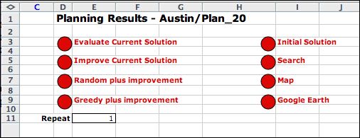
Buttons |
| |
At the top of the page there are
several buttons. The first button on the left evaluates the
current solution. If the sequence is changed in column E, click
this button to see the results of the change. The second button, Improve
Current Solution, uses insert, switch and turn heuristics
to improve the solution. The third button, Random plus
improvement option generates a random solution and improves
it to a local minimum. The Greedy plus improvement option
generates a greedy solution and improves it to a local minimum.
The first button on the right creates the feasible initial
solution. The Search button opens a dialog that allows
the specification of more complicated search options. The Map button
creates a worksheet with a map of the current solution. The Google
Earth button
creates a program the is used to show the solution on the Google
Earth application. This button only appears when locations
are given geometric coordinates.
The cell E11 allows the heuristic to be run several times
in succession. It is only effective for one of the improvement
options that involve random starts. For example if the repeat
number is set to 10 and we choose the Random plus Improvement option,
the improvement process is carried out ten times. If more than
one local optimum is reached. The solution found is the best
of these.
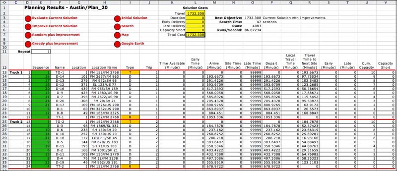
To illustrate the improvement process we choose
the Random plus Improvement button. The results are
shown below. Click the figure to see a larger illustration. The
first truck visits delivery sites 14, 13, 12, 16, 9, 7, 20, 17, 1, and 8. The
second truck visits sites 3, 6, 10, 18, 5, 15, 2, 11, 4, and 19. There is no
shortage in the capacity, since each truck makes 10 deliveries. The
sequence of trucks and deliveries defines the two trips. There may be better
solutions than this one since a heuristic solution cannot guarantee
the optimum. |
|
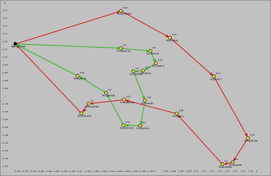
Map |
| |
Clicking the Map button creates a map
showing the two trips. Trips routes between map locations are
colored green and red. Delivery
locations are yellow and truck locations
are black. |
|
| |
There is no guarantee that this
is an optimum solution. The multiple vehicle routing
problem is a hard problem. There are optimization models that
can assure optimality, however, large problems may lead to
prohibitive computation times even on powerful computers.
On a later page we show examples of this problem with other
parameters, but the next page considers the model worksheet. |
| |
|
|