|
|
The vehicle routing problem is
a combinatorial problem. For a problem of even moderate size,
the number of feasible solutions is finite but very large.
There is no known algorithm that can determine optimal solutions
for very large problems. We cannot hope to solve meaningful
problems with the Excel based optimization tools in the ORMM
collection, so we seek good solutions with heuristics.
The VRP is represented as a sequencing problem. The
sequence gives an ordered list of nodes representing truck
and delivery locations. Each truck contributes two nodes to
the problem, one for leaving and one for returning, and each
delivery contributes one node. Starting from an initial sequence,
candidate solutions are discovered by applying various heuristics
to the sequence. The goal of each heuristic is to reduce the
cost associated with the sequence. The cost model is implemented
on the Model worksheet. When the process is complete a solution
is obtained that is generally much better than the starting
sequence, but there is no guarantee of optimality. The final
sequence provides an upper bound to the optimum objective.
No lower bound is provided by our methods, so there is no measure
of quality. That
is an inherent disadvantage of purely heuristic approaches.
Although we believe that meaningful problems can be solved conveniently
by this Routing add-in, the add-in cannot compete with the computational
methods that have been designed and demonstrated by others. The
Vehicle Routing problem (VRP) and the related Traveling Salesman
problem (TSP)
are perhaps the most studied problems of Operations Research.
One of the first computer solutions was demonstrated in 1954 with a solution
of a 49 city problem that passes through every state in the continental USA
and Washington DC. Great progress has been made during the 50 years since this
problem was introduced. At the date of this writing, a TSP with over 85,000
nodes has been solved to optimality. The excellent Traveling Salesman Problem
web site (http://www.tsp.gatech.edu/)
describes this problem as well as many other interesting facts
about the history of the TSP.
In the following we use the term nodes to signify both truck and delivery
locations. Since the example uses Euclidean metric to compute distances
between two adjacent nodes. The distance is independent of the order in which
two nodes appear in the sequence. When the time aspects of the problem are
ineffective, the associated routing problem is said to be symmetric.
Although heuristics can be adapted to take advantage of symmetry, our add-in
does not. Our interest is to make the solution process as general as possible.
For this page and the next we use a problem from the routing_demo.xls |
Solutions with One Truck |
| |
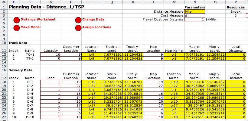
We illustrate the solution methods first with
a TSP that is represented as a VRP with a single vehicle
(truck). The data for the problem is on the TSP data worksheet
shown below. The time feature is not included in the example.
The capacities and loads in column G are set so that the single
truck must serve all the deliveries. The map locations in column
O refer the map indices shown earlier and are assigned randomly.
The truck begins and ends its route at location 9. The deliveries
are at various map locations. Coordinates for the locations
are obtained from the distance worksheet. The truck
and delivery (site) coordinates are the same as the map coordinates,
so local distances are zero. The data chosen makes the problem
equivalent to the TSP problem where the cost of a solution
is equal to the total distance traveled by the single delivery
truck. |
|
| |
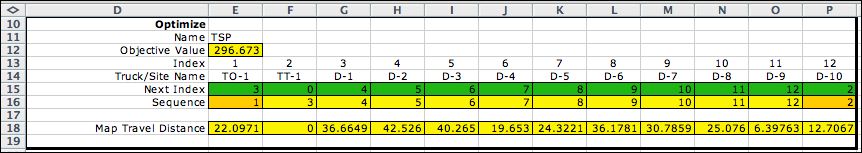
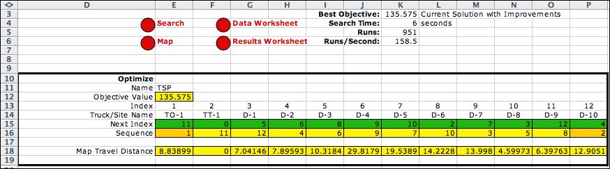
The figure below shows the initial solution
for the problem one the model worksheet. Cell E12 holds the
objective function computed for the solution. The green cells
in row 15 describe the current sequence by indicating the
next site to be visited from each node. The yellow cells in
row 16 hold the sequence of nodes on the truck's path. The
yellow cells in row 18 compute the Euclidean distance between
adjacent nodes on the sequence. For the simplified data of
the example, the sum of the values in row 18 is the same as
the objective value in E12. The goal of the optimization is
to find the solution (row 15) that minimizes the objective
value in E12. |
|
| |
We choose this initial solution because it
is easy to find. From row 16 we see that the truck starts at
node 1, travels sequentially to nodes 3, 4, ...12, and finishes
at node 2. Node 1 is the origin for the trip taken by the truck
(TO-1) and node 2 is the terminal node for the trip (TT-1).
The solution in row 15 shows the sequence in a less direct
way. The sequence always starts at node 1. To find the next
node in the sequence we look in cell E15 to find the node 3.
To find the next node in the sequence we must look at G15,
to find the value 4. The process continues until the sequence
is complete. Cell P15 indicates a return to node 2, the terminating
node for the truck. A feasible sequence with
one truck must start at node 1, visit each delivery site
once and only once, and finish at node 2. |
| |
| Rows 15 and 16 describe the trip in two different ways.
The variables for the problem are in row 15. The sequence
in row 16 is computed by Excel formulas that depend on
row 15. Our heuristic solution methods manipulate the sequence
by changing row 15. Notation for the next-index
vector and the sequence vector are shown at the right. |
|
| Given the variable row (15), the sequence row (16) is computed
recursively with the formulas at the right. |
|
| Given the sequence row (16), the variable row (15) can
be computed recursively with the formulas at the right. The
model does not use these formulas. The model sets the variables
in row 15 and computes the variables in row 16. |
|
|
| |
After a series of heuristics is applied to the
initial solution, we obtain the TSP
solution illustrated below. Optimality cannot be guaranteed,
but the heuristic methods usually
find the optimum for small problems. Column
K shows statistics for the solution process. |
|
| |
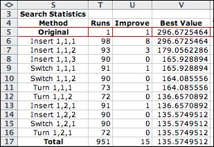
The heuristics used in the process are
listed at right.
For each heuristic, column T indicates the number of objective
function evaluations (called runs), column U shows
the number of the runs that result in improved objective
values, and column V shows the best value of the objective
obtained. For the case illustrated, 951 solutions were evaluated.
Fifteen of the evaluations showed improvement in the objective
value. The best values in column V decrease from the value
of the original sequence to the value of the final sequence.
The next page describes the heuristics. |
|
|
| |
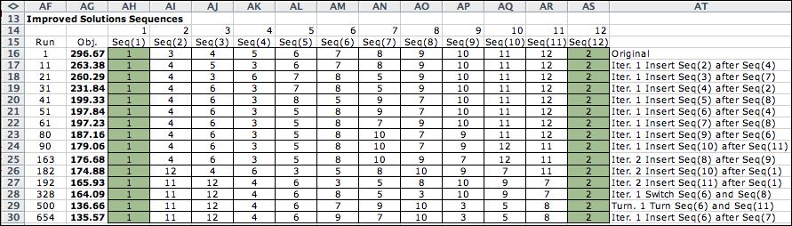
A list of the improving sequences is shown below
the model. |
|
| |
The maps showing the initial and final solutions
are below. The truck location is the black node and the delivery
locations are red nodes. |
|
Solutions with More than One Truck |
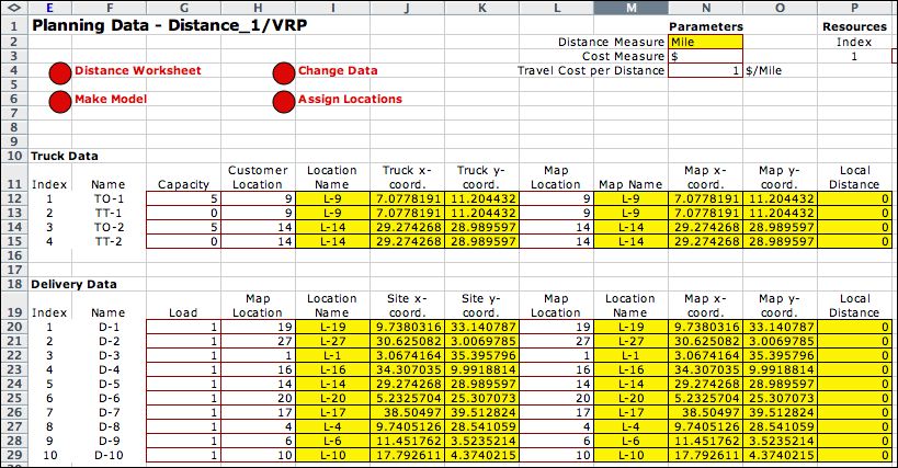
| |
We use the same example with two trucks to illustrate
the multi-vehicle case. Each truck has two rows of the data table,
one for the origin node of the truck trip and one for the terminal
node. The origin and terminal nodes need not be the same, but
they are in the example. The entries in column N serve to partition
the deliveries between the two trucks. Each truck serves five
delivery locations. |
|
| |
The initial solution is show below. The origin
and terminal nodes for truck 1 are indexed 1 and 2. The origin
and terminal nodes for truck 2 are indexed 3 and 4. The
initial solution for the multi-truck problem has all but one
truck node at the beginning of the sequence and the terminal
node of the last truck as the last. The deliveries are listed
in index order before the terminal node of the last truck. For
any given truck, the nodes between the origin node and the terminal
node describe the trip for that truck. The solution below shows
the first truck with no deliveries, while the second truck
has them all. |
|
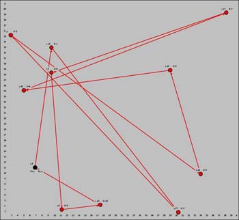
| |
The model penalizes solutions that are infeasible
with respect to resources. The second truck violates the constraint
because the capacity of truck 2 is five deliveries and the
sequence requires the truck to make ten deliveries. The solution
process will eliminate this infeasibility as it attempts to
minimize the objective function.
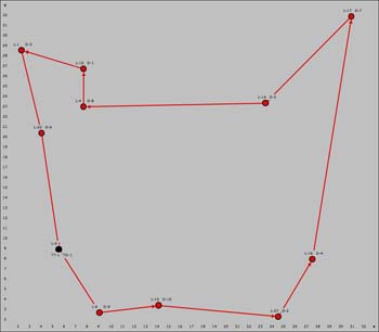
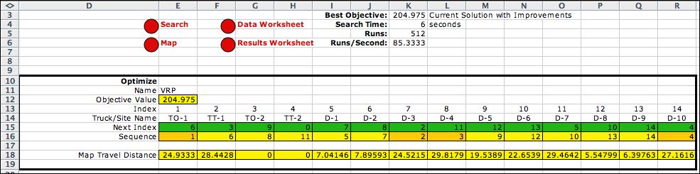
After a series of heuristic changes, we obtain the solution
below. The solution illustrates a requirement for feasible
solutions for the multi-truck problem. Except for the last
truck, the originating node of the next truck must immediately
follow a terminating truck node. Row 16 shows that node 2,
the terminal node of truck 1, is immediate followed by node
3, the originating node of truck 2. The sequence begins with
the originating node of truck 1, and it ends with the terminal
node of truck 2. The nodes between the original node and terminal
node describe the sequence of deliveries for each truck. Again
we cannot guarantee optimality. |
|
| |
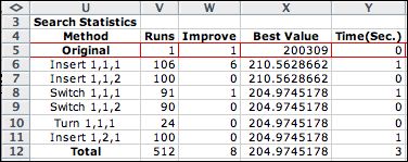
The heuristics used in the process are listed at the
right. The method required 512 runs. Only eight of the
runs showed an improvement. |
|
|
| |
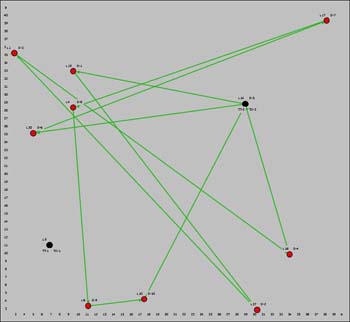
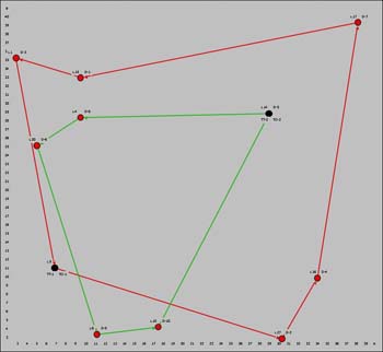
The initial and final maps are below. The two
trips are shown with different colors. The truck locations are
colored black and the delivery locations are in red. |
|
The Number of Feasible Solutions |
| |
The number of feasible solutions depends on the
number of trucks and the number of deliveries. The number of
truck nodes is equal to two times the number of trucks. The first
and last nodes in the sequence are fixed and are both truck nodes.
The remaining truck nodes are moved as a pair, so only half of
these nodes count toward the number of solutions. The total number
of feasible solutions is the factorial of the number of free
nodes. |
| |
|
| |
For the small example with two trucks (four
truck nodes), the total number of feasible solutions is the
Factorial of 11. This number is over 39 million. Exhaustive
enumeration of all feasible solutions can find the globally
optimal solution, but this method can be used for only very
small problems. |
| |
| Number of Truck nodes |
4 |
| Number of Delivery nodes |
10 |
| Number of sequence nodes |
14 |
| Number of free nodes |
11 |
| Number of Solutions |
39916800 |
|
| |
The next page describes the heuristics used to
search through the solution space to find good solutions in
practical
computation time. |
| |
|