|
|
Most people when dealing with
some problem want the optimal solution. When optimization
is impractical, heuristic methods are necessary. Heuristics
use some characteristic of the problem to direct a search for
a good solution. The possibility of finding the optimum is
remote,
but successful heuristics often deliver a satisfactory solution.
A variety of heuristics have been proposed for the TSP and
VRP. We use the three heuristics described on this page.
Every heuristic starts with a base sequence: S =[s(1), s(2), s(3)... s(n)]
with objective value Z. The heuristic suggests changes
in the base sequence to obtain a different sequence, S' =[s'(1), s'(2), s'(3)... s'(n)]
with objective value Z'. The goal is to find a sequence
with a lower objective function value, Z' < Z. A
heuristic method applies one or more heuristics until no further
improvement is possible. The point reached is a local optimum.
Heuristics have a long history with regard to the solution
of the TSP and related problems. A site by Steven
Mertens provides
animated examples. |
Local Optima |
| |
A heuristic starts with a given sequence and
changes the sequence in some prescribed way. We call
a change a move. The set of possible moves from
a given solution is limited and the set of all solutions reachable
via the move is called the neighborhood. A greedy
heuristic accepts only moves that improve the objective value.
Starting from an initial sequence, we use a greedy heuristic to
move through a series of solutions until a solution is reached
where no further improvement is possible. There must be a finite
number of moves in an improving sequence since the solution space
is finite. The solution reached is called a local optimum.
The global optimum is the best of all local optimums. |
Insert Heuristic |
| |
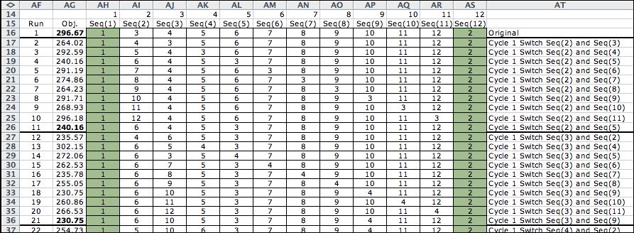
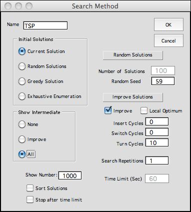
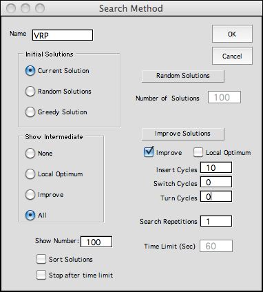
To illustrate the Insert Heuristic we
start from the default initial solution and click
the Search button
from either the Results or Model worksheet.
The Search button
offers the alternative to show the sequences considered by
the add-in. In the dialog select the Improve option
and specify a large number of Insert Cycles. Clicking
the All button on the Show Intermediate frame
will create a list of all moves encountered during the process.
The list is illustrated below.
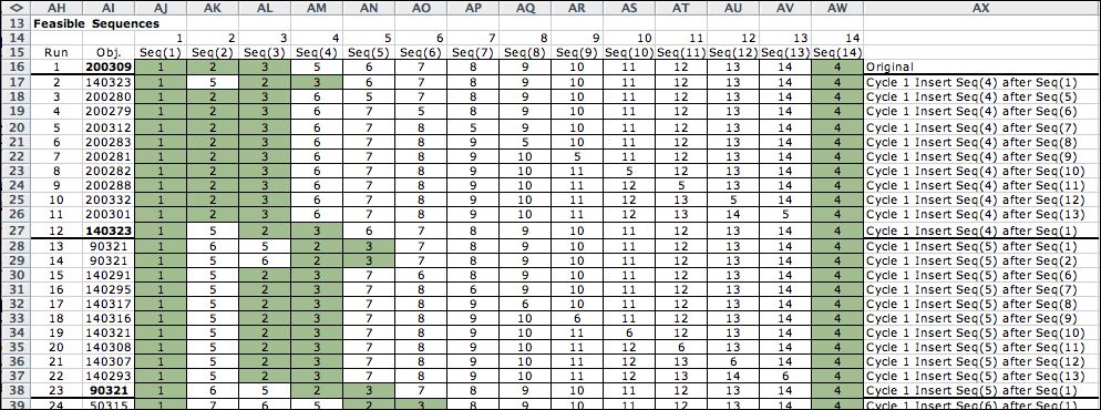
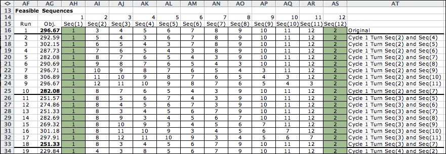
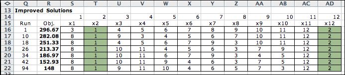
The insert heuristic is to remove one node from
the sequence and put it in a different place.
The figure
below shows a series of insert moves. The sequence at the
top is the initial base sequence, S. This simply
lists the deliveries in order. Run 1 removes the node at
position 4 (s(4) = 5) and places it after position
1. The changed sequence will have s'(2) = 5. The
change requires other positions in the sequence to change, s'(3)
= 2 and s'(4) = 3. The objective value is computed
and shown in column U. The new sequence is shown as
run 2.
Runs 2 through 11 all begin from the base sequence
and move the contents of position 4 to other positions
in the sequence. After all possible relocations of s(4),
we note whether there has been an improvement over the
base sequence. If so, the best of the 10 observations becomes
the base sequence. For the example, run 2 provides the
most improvement, so the new base sequence is shown as
run 12.
Our add-in changes the base sequence based on the best
move from a particular location. A different implementation
might change the base sequence whenever an improvement
is discovered. There are many ways to implement a given
heuristic and it is hard to say which is better. |
 |
|
|
| |
The process continues by moving s(5)
to other positions. The best of the moves evaluated in runs
13 through 22 is run 13. The new base sequence is run 23.
Moves are restricted so that only sequence members that currently
hold delivery
nodes, rather than truck nodes, are considered for movement.
For the base sequence of run 1, this rule excludes s(1), s(2), s(3),
and s(14)
from moving. The truck nodes may shift due to
other moves. The restricted members are shown in green in the
sequence list. Also the insert location must not currently
hold a node representing
a terminal node of some truck. For run 1 of the example, s(4)
can be inserted after s(1),
but not after s(2).
The
objective values for the base sequence improve as the runs
progress. A complete cycle of the insert heuristic examines
all unrestricted moves. The cycle illustrated partially
above required 107 runs.
Six of these resulted in improvement. Improvement moves are
evaluated
twice. One additional insert cycle was run where no improvement
was observed. The second cycle required another 100 runs.
Insert moves are restricted so that the s(1) and
s(14) remain the same and the truck terminal and
origin pairs are not separated. Thus we see that nodes 1 and
12 are
always at the extremes of the sequence and nodes 2 and 3 remain
together.
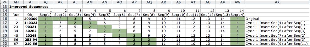
An alternative presentation shows only the runs that improve the objective
value. |
|
| |
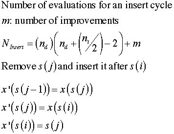
Every sequence has an equivalent vector
of next indices, X.
Each insert move requires only three changes of X. The
formulas for the changes are at the right. The change for
run 12 removes s(4) and inserts it after
s(1).
The add-in implements an insert move by changing
three values in the X vector on the Excel worksheet.
The objective function value is calculated directly with
the formulas on the worksheet. The number of objective
function changes for a complete cycle of the insert move
is approximately equal to the square of the number of delivery
nodes.
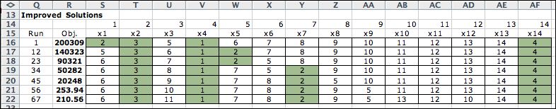
Each row of the table below shows the X vector
for an improving solution. |
|
|
|
| |
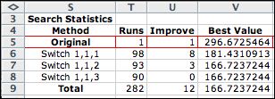
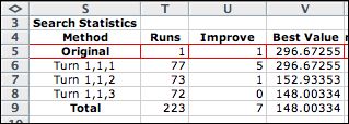
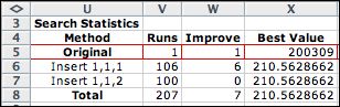
Although the dialog called for 10 cycles,
the algorithm terminates when a cycle results in no improvement.
The statistics at the right show six improvements during
the first cycle and none in the second. The result is a local
optimum for the insert heuristic.
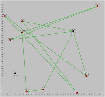
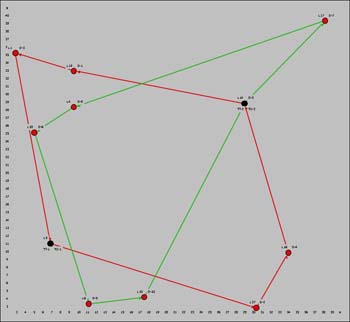
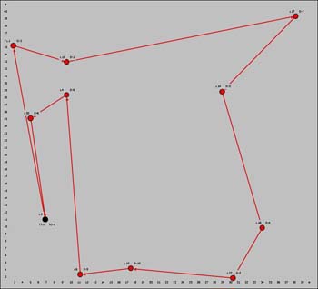
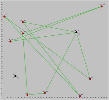
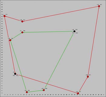
The initial solution is compared with the map after two
insert cycles. The initial solution uses only one truck.
The insert moves divide the deliveries between the two
trucks. |
 |
|
Initial Map |
Map after insert cycles |
|
|
|
|
| |
For this section we consider the TSP problem
on the demonstration worksheet. This model has only one
truck represented by the first and last nodes of all sequences.
To illustrate the Switch
Heuristic we
again start from the default initial solution and click
the Search button
from either the Results or Model worksheet.
In the
dialog select the Improve checkbox and specify
a large number of Switch Cycles. Clicking the All button
shows all sequences encountered.
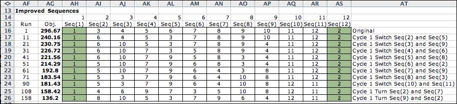
A switch move involves two delivery nodes. The move is
accomplished by switching the contents of two sequence
positions. We use as an example the TSP that routes a single
truck through 10 delivery locations. The initial base sequence
is row 1 below. The move reported in run 2 switches s(2)
and s(3). The changed sequence has
s'(2) = s(3) and s'(3)
= s(2).
The first step of the switch cycle reviews
the ten possible
switches and reports the best as run 11. A cycle is complete
when all nodes have been reviewed for a switch. |
|
|
|
| |
A local optimum is reached after three cycles. The last
cycle indicates that no further improvement is possible.
Only the
improving moves are shown in the table below. |
|
|
| |
|
| |
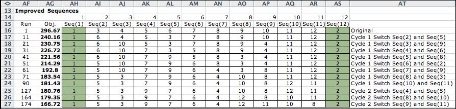
The switch move involves only delivery nodes
and each cycle evaluates switching every sequence component
with all other components except itself. A cycle
of switch moves evaluates all possible moves. The number
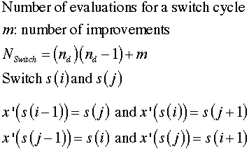
of switches is given by the formula at the right.
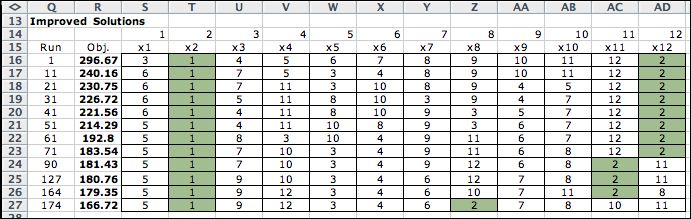
Each sequence has a corresponding next-index
vector. The example runs are shown below. Four changes
are necessary for a switch move involving nonadjacent sequence
values. The changes for run 11, switching s(2)
and s(5),
are:
s(1)=1, s(2)=3, s(4)
= 4, s(5)=6
x'(1) =6 , x'(2)
= 3, x'(5) = 3, s(6) =1.
The next-index vectors are shown below. |
|
|
|
| |
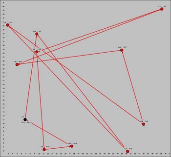
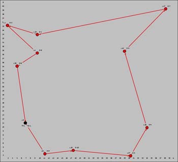
The maps showing the initial and final solutions
are below. The truck location is the black node and the delivery
locations are red nodes. |
Initial Map |
Map after switch cycles |
|
|
|
Turn Heuristic |
| |
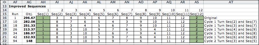
This heuristic selects two nodes in the
sequence. The sequence locations of the two nodes are switched
as in the switch move. The turn move then reverses
the path between the two nodes. The move is equivalent
to turning around a path in the directed graph described
by the base sequence. Thus we call this the turn heuristic.
For the TSP, a turn cycle reviews all paths in the base
sequence and evaluates the objective function. For the
VRP we require that both ends of the path reside on the
same trip. Nodes representing the origin or terminal node
for a truck are not affected by the turn move. The move
does not consider paths formed by two adjacent nodes. Such
a move is equivalent to a switch move that involves
adjacent sequence locations.
Run 1 in the figure below selects the path (3, 4, 5) and
turns it around to form the path (5, 4, 3). The heuristic
considers all pairs of sequence elements such that the
first element is in a lower position than the second. |
|
|
|
| |
| The display showing only improving sequences is shown below. |
|
|
|
| |
For the TSP the number of evaluations in
a cycle is again of the order of the square of number
of deliveries. For a VRP the number is less because
paths cannot include truck nodes.
This move involves more elements of the sequence and next-index
vectors, so we do not attempt to write general formulas
for this heuristic. |
|
|
|
| |
The various heuristics can be combined. When the
turn cycle is performed after a switch cycle, the turn
cycle operates on the base sequence provided by the switch cycle.
In the example below, the first 8 sequences are switch
moves and the final two are turn moves. |
|
| |
The turn move can be described by several
insert or switch moves, but since the heuristics are performed
one move at a time, beneficial turn moves are often missed.
The example shows the effect of two turn moves applied to the
sequence found with the switch move. |
Map after one switch cycle |
Map after turn cycles following
switch cycles |
|
|
|
Strategies |
| |
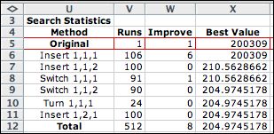
It is unlikely that a single heuristic method
will yield a very good solution. The add-in allows
strategies that combine the three heuristics
described on this page. Clicking the Improve Current
Solution button
on the Results page prepares a strategy that repeats
the three strategies, insert, switch and turn, until all
three heuristics result in no additional improvements. The solution
obtained is a local optimum for the combination of heuristics. |
|
|
| |
The initial and final maps are below. The two
trips are shown with different colors. The truck locations are
colored black and the delivery locations are red. The final
map is probably the optimum solution, but with heuristics you
can't be sure. |
|
More Strategies |
| |
Many heuristics have been proposed in the literature
for TSP and VRP problems, including Tabu Search, Simulated
Annealing, and Genetic Algorithms. A Google
search will reveal web sites about each of these and others.
They all attempt to evaluate a relatively small number of solutions
to identify a good solution. The methods used by the Routing
add-in are among the simplest.
All the heuristics discussed on this page are
greedy heuristics. The insert, switch and turn heuristics accept
improving moves until no improvement can be obtained. A solution
found in this way is called a local optimum. The solution depends
on the initial sequence. One way to improve the solution
is to start the process at several different initial sequences
and select the best of the final solutions. The add-in
has tools to prescribe strategies of this kind. They are described
on the next page. |
| |
|