|
|
 |
Vehicle
Routing |
 |
-
Strategy |
|
|
The heuristics on the last page
are applied in cycles. All three heuristics consider node pairs
where the application of the heuristic changes
the sequence in some manner related to the pair.
There are restrictions on changes that assure that
the truck nodes remain in the same order as in the initial
solution. Given the initial base sequence, we select
the first node and then
evaluate
the objective function for every choice of the second node.
If one or more of the pairs result in improvement of the
objective value, the best pair is applied to the base
sequence to form a new base sequence. The process continues
until all nodes are considered as the first node. This is called
a cycle.
Since only
improving pairs
are accepted for implementation, the objective value for the
base sequence always declines. If there is no improvement for
a cycle, the process stops because no further improvement is
possible using the current heuristic. The process then terminates
or continues with a different heuristic.
A strategy involves selecting the order of applying the heuristics
and determining how many cycles to run. A deterministic heuristic
carried to the point where a complete cycle shows no improvement
leads
to a local minimum. To investigate alternative local optima,
we use two different methods for selecting starting solutions
randomly.
The example for this page has 20 deliveries with four identical
trucks. Time is not part of the model, so the goal is to
minimize total route length. Four trucks are used in the example
and each truck is required to make five deliveries. The data
is on the Routing_20.xls demonstration
file. |
Strategy Components |
| |
A strategy consists of a combination of heuristics.
The candidate components for a strategy are listed in the table
below. The process always begins with the solution on the result
worksheet. Strategies are evaluated in the Sequence Optimizing add-in
that manipulates solutions on the model worksheet. After the
completion of the optimization process, the solution is transferred
from the model worksheet
to the results worksheet. The initial solution must define
a valid sequence.
It is possible to set the initial solution manually on
the results worksheet.
The default values for the number of cycles are in the last
column. NS is the number nodes sequenced (2*trucks + deliveries).
The search process may use a specified number of cycles or
allow as many cycles as necessary to reach a local optimum
for each heuristic. For a local optimum for the process, the
search process uses as many cycles as necessary until a cycle
results in no improvement for every heuristic.
Component |
Definition |
Default Value |
Original |
The sequence defined when the search process
is initiated |
1 |
Random |
The set number of randomly generated initial solutions |
1 |
Greedy |
The set number of greedy solutions with the initial solution randomly
generated |
1 |
Insert |
The number of cycles of the Insert heuristic |
3 + Int(NS / 10) |
Switch |
The number of cycles of the Switch heuristic |
3 + Int(NS / 10) |
Turn |
The number of cycles of the Turn heuristic |
2 + Int(NS / 10) |
Replication |
The number of replications of the Strategy |
1 |
Optionally, the Random or Greedy procedures
will generate a specified number of solutions. The best of
these randomly generated sequences and the original solution
determines the starting solution for the remaining heuristics.
The Insert, Switch, and Turn heuristics follow
in order. Each heuristic is applied for a specified number
of cycles unless a cycle has no improvements. If a cycle leads
to no improvement, the heuristic is terminated allowing the
next heuristic to begin. The specification of the Random or Greedy heuristics
plus the numbers of the cycles for the remaining heuristics
determine the strategy. If the local optimum checkbox
is clicked the sequence number is neglected. |
| |
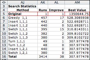
The Replication input allows strategies
to be run more than once. When a randomized starting solution
is used, it is best to run several replications of the strategy
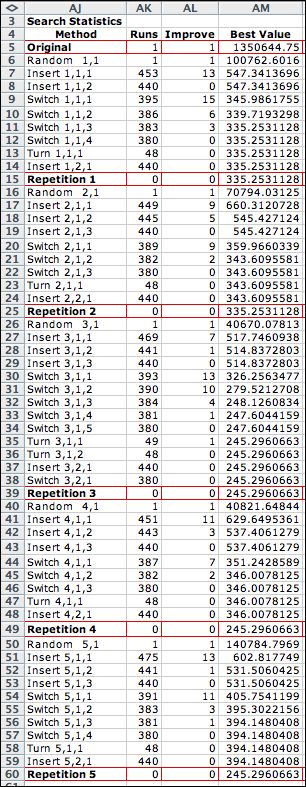
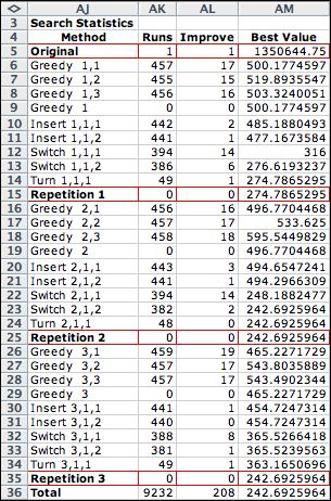
and choose the best of the local optima. The figures on
the right shows the results of six repetitions of the strategy
that begins with a random solution and continues through
cycles of the insert, switch and turn statistics. Each
repetition stops with a local optimum. The titles in column
AI of the display are followed by one to three integer
numbers. The first number is the repetition number, the
second is the number of times the heuristic type has been
visited during the strategy, and the third number is the
cycle number within the visit.
Replication
summaries are displayed on the Models worksheet
as illustrated at the right. Columns identify the heuristic
or initializing method, the number of runs, the number
of runs finding improved solutions and the value of the
best solution after the starting process or heuristic has
been performed. (The time and run/second statistics are
also shown on the worksheet, but not illustrated here.)
Row 5 shows the initial solution and rows 6 through 14
show the first replication. The replication begins with
a single random solution in row 6. The first two cycles
of the Insert heuristic,
in rows 7 and 8, result in 13 improved solutions, while
the third shows no improvement. Two cycles of the Switch heuristic,
in rows 10 and 11, yield 21 improvements, while the last
in row 12 has none. The single turn cycle in row 13 shows
no improvement. One more insert cycle is required to meet
the requirement for a local minimum. When three heuristics
are used, three consecutive 0's in the Improve column indicate
a local optimum.
The objective value in row 14 is the objective value for
a local optimum solution. Row 16 compares this solution
to the value of the best solution obtained in the previous
replications or the original solution.
Other replications repeat in like manner. Since all begin
with different random initial solutions, each may terminate
with a different local optimum. The Best Value column in
rows 14, 24, 38, 48 and 59 are all different indicating
that four local optimum solutions have been discovered.
The best of these is in row 38.
|
|
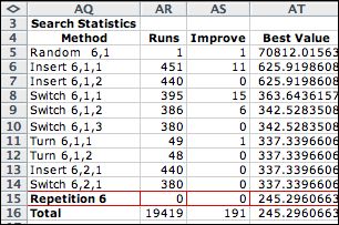
The last replication is reported
in a new column to avoid overwriting other contents on
the worksheet. We see one more local optimum values in
row 14.
The Total row reports 19419 runs
with 191 improved solutions. The best solution has
the value of about 245. The decision values and sequence
values are reported on the model and result worksheets. |
|
|
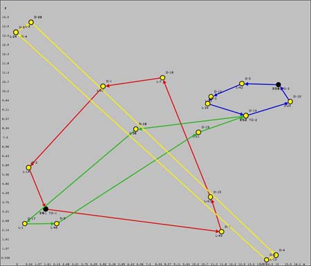
Local Optimum Solutions |
| |
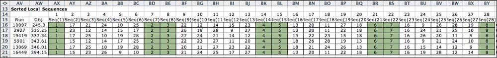
The sequences for six local solutions found during
the search are
shown below. Using the selected strategy, none
of these solutions can be improved. The solutions are sorted
by their objective values with the best on top. |
|
| |
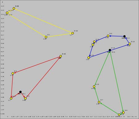
The best and worst or the six local optima
are shown in the figures below. The best solution (on the left)
looks reasonable. The worst (on the right) illustrates the
problem of heuristic solutions. It is
not
hard to see that the yellow trip is not advisable, but no
single
change can improve it. There are several ways to reduce the
problem of local minima including:
heuristics that sometimes accept non-improving moves, solving
the problem to optimality as an integer program, and solving
the problem with a large number of random initial solutions and
selecting the best local optimum. All of these solutions increase
the computational cost
of finding good solutions. The only available solution for this
add-in is to use many repetitions of the strategy. Later versions
of the add-in may investigate the other options. |
| |
|
Built-in Strategies |
| |
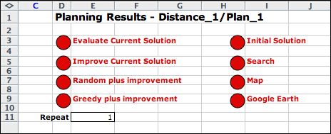
The buttons on column D of the Results worksheet
initiate several built-in strategies. The Repeat field
specifies the number of replications for the strategy.
The first two buttons on the left are not affected by the
number in this field, but multiple replications are useful
for the last two strategies that involve random initial
solutions.
The first button in column D evaluates the current solution
without searching for a better solution. This might be
useful when the analyst is adjusting a solution determined
by the add-in. The current sequence is defined by the entries
in column E of the Results worksheet.
When the button is clicked, the sequence is transferred
to the Model worksheet to evaluate the solution.
Computed results on the Model worksheet are subsequently
transferred back to the Results worksheet. The
user-defined sequence must have no loops and must have
a unique index in each row of column E.
|
|
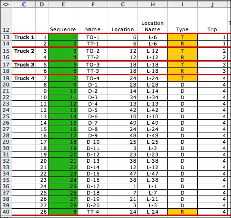
The buttons on the right side (column H)
call VBA subroutines. The Initial
Solution button
creates a simple solution for the VRP problem illustrated
at the right. The initial sequence is in column E. The example
has four trucks and for the initial solution truck 1 through
3 have no deliveries, while truck 4 has them all. In general,
when the plan has several trucks, the last truck handles
all the deliveries. The route through the deliveries is determined
by the delivery indices. This is usually not a good solution,
but it provides a convenient starting point for illustrating
the various options.
The Search button provides for a user-defined
search as described below. The Map button creates
a worksheet mapping the coordinates of the trucks and deliveries
and displays the route in column E. The Google Earth button
helps to create a Google Earth display of the results. This
is described on a later page of this section. |
 |
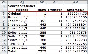
The Improve Current Solution button
on the left seeks a local optimum solution starting from
the sequence in column E. The statistics on the right are
for the simple initial solution pictured above. Only two
insert cycles are used because the second insert cycle
made no improvement. Three switch cycles, and a turn cycle
completes the first replication. Since improvements occur
after the insert cycles in rows 6 and 7, a second replication
begins in row 12. The process is terminated when that cycle
provides no improvement. It is interesting that this solution
is better than the best found with six random starting
solutions.
|
|
The Random Plus Improvement button
generates a random solution and improves that solution
to a local optimum. The random solution value is in row
6.
The final solution is a local minimum. |
|
The greedy initial solution is
constructed in a manner that usually results in a better
solution than a random start. As for the simple initial
solution the first 3 trucks are assigned no deliveries
and the last truck has all the deliveries. Rather than
list the deliveries in order of index as for the simple
initial solution, the greedy solution selects
a random
order for the deliveries. Then a cycle of the insert heuristic
considers each delivery in order and places it in the
position that most improves the objective value. Since
this is a one-pass greedy process, it rarely obtains even
a local optimum, but it leads to better initial solutions
than
a purely random start mechanism. In the example the result
is reported in row 6.
The improvement strategy is then applied to obtain a
local optimum. For the example, the final solution is even
worse than the random start. There is no guarantee that
a better initial solution leads to a better final solution.
Multiple replications are allowed for this option. |
|
|
User-designed Strategies |
| |
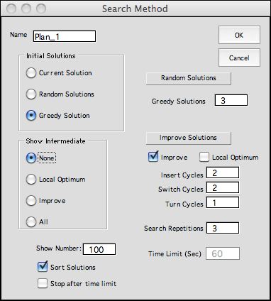
Clicking the Search button
at the top of the Results or Model worksheets
presents a dialog for choosing the strategy. The dialog below
selects a greedy start that is the best of three random greedy
solutions (the top field on the right). Clicking
the Improve check box on the right without checking
the Local Optimum check box allows cycle numbers to
be specified for the strategy. The heuristics are always applied
in the order insert, cycle and turn, but different numbers
of cycles may be entered, including 0. The search replication
box is set to 3. The search activity is detailed starting in
column AI. Each replication begins with the best of three greedy
solutions and continues until either the desired number of
cycles has been performed or local optimums are obtained. Since
optimality conditions are not satisfied, the solution of a
replication may not be a local optimum, although in this case
it was shown to be local optimum earlier on this page.
We provide the Search option to allow student experimentation
and to test alternative strategies. For a large problem it
might be better to select the number of cycles, because the
solution time is not easily bounded for the
local optimum option.
|
| |
A variety of strategies are available through
the algorithm. There is no limit to the size of the problems
that can be solved with the add-in except as limited by the
number of columns on the Excel worksheet. Of course larger
problems require more solution evaluations to reach quality
solutions and heuristic cycles use
more time. Excel with the Routing add-in is not a
competitor to commercial programs or more efficient algorithms
running on powerful computers, but this tool may have value
to students and to small organizations. |
| |
|
|