|
|
 |
Vehicle
Routing |
 |
-
Model |
|
|
The Model worksheet is
entirely constructed by the Routing add-in. Its purpose
is to collect data from the Data worksheet,
interact with the search algorithms in the Optimize
Sequence add-in, and report solutions on the Results worksheet.
Although users familiar with the add-ins
may experiment by changing some features of this worksheet,
in general it is better to leave it alone.
In the following we divide the model worksheet into three
parts to simplify the discussion. The parts are different in
function. The particular
solution shown in the example is the same one illustrated on
the Results page. |
Optimize Model |
| |
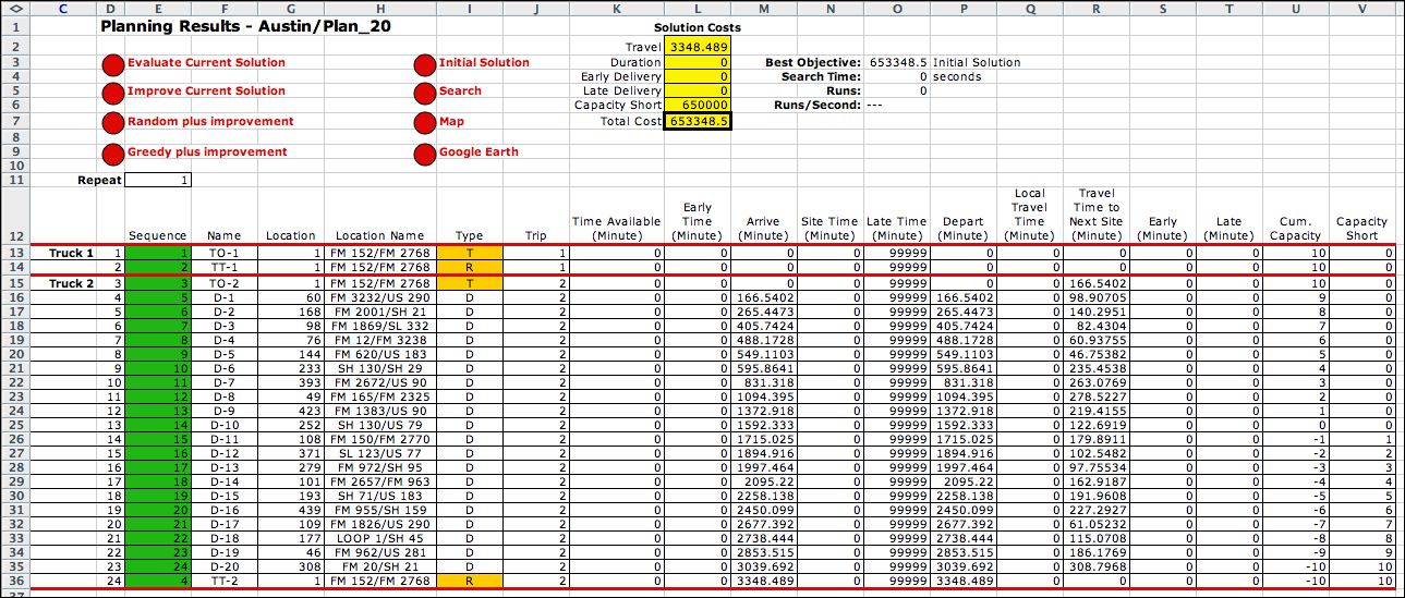
At the top of the model worksheet
shown below are the control buttons and the results of the
most recent computation. Rows 10 through 19 hold the decision
variables, the objective function, the current sequence and
the distances between map locations. A similar form is constructed
by the Optimize add-in
as described on the Combinatorial
Form page. The form is particularly adapted to the TSP on
the Traveling
Salesman page. Here we adapt the TSP form for
the routing problem.
For this model we identify the items to be sequenced as nodes.
Each node is related to a truck origin node, a truck
terminal node or a delivery site. The nodes referring to trucks
are indexed first. For example with two trucks, the first four
nodes are TO-1, TT-1, TO-2, and TT-2. The last ten nodes relate
to delivery sites, nodes 5, 6, ... 14 refer respectively to
D-1, D-2, ... D-10. This one-to-one assignment does not change
during the solution process. The relationships between nodes
and the routing problem elements are stored on the Excel worksheet
in rows 13 and 14.
We seek the sequence of nodes that gives the smallest value
to the objective function in cell E12. E12 holds a formula
that evaluates the complex cost model described on the remainder
of this page.
There are some rules concerning acceptable
sequences. The first rule is that the first node of the sequence
represents the origin node of the first truck. For the example,
node 1 representing TO-1 must begin the sequence. The second
rule is that the last node of the sequence must represent the
terminal node of the last truck. For the example, node 4, representing
TT-2, must end the sequence. Further wherever a truck terminal
node appears in the sequence, the origin node of the next truck
must follow. We see this in the figure where the terminal node
for truck 1 appears as the 7th node in the sequence. The origin
node of truck 2 must be the 8th node of the sequence.
This assures that every delivery is handled by exactly one
truck. The enumeration
process maintains these relationships.
Row 15 describes the sequence by indicating for each node
the next node in the sequence. We see in E15 that node 13 (D-9)
follows node 1 (TO-1). In Q15 we see that node 9 (D-5) follows
node 13 (D-9). This process can be continued to find the complete
sequence. The entries in row 15 are the variables of the problem.
They are controlled by the program that implements the heuristic
solution process.
Row 16 describes the sequence more directly by listing the
nodes in sequence order. E16 holds the first node in the sequence,
node 1 (TO-1). F16 holds the second node in the sequence, node
13 (D-9). G16 holds the third node in the sequence, node
9 (D-5). The process continues until the last node in the sequence
is reached. This is node 4 representing the terminal node of
the second truck,
TT-2. Row 16 is computed with Excel formulas
from decisions in row 15.
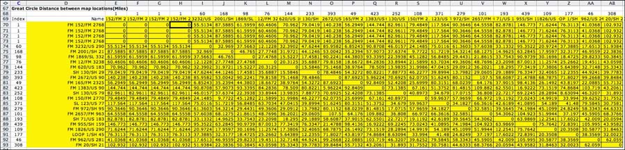
Row 18 holds the map distances between the locations of adjacent
nodes in the sequence. For instance the value of E18 is the
distance between the location of node 1 and the location of
node 13. For the example, the location of node 1 is L-9, and
the location of node 13 is L-6. E18 is the distance between
L-9 and L-6. The numbers in row 18 are Excel lookup functions
that reference a matrix further down on this models page. |
|
| |
For
the example, the sequence is (1,
13, 9, 8, 6, 14, 2, 3,
11, 5, 7, 10, 12, 4).
The colored indices in the sequence are nodes related to
the trucks. The particular sequence defines the route (1,
13, 9, 8, 6, 14, 2)
for truck 1. The route begins at the origin location of truck
1 and ends at the terminal location of truck 1. The route for
truck 2 is (3,
11, 5, 7, 10, 12, 4).
It begins at the origin location of truck 2 and ends at the
terminal location of truck 2. The travel distances associated
with the links of the trip are selected from the distance matrix
using a LOOKUP equation. For example, the value, 8.83899,
in cell E18 is the Euclidean, or straight-line distance, from
node 1 to node 13. The other entries in row 18 are
similarly computed. |
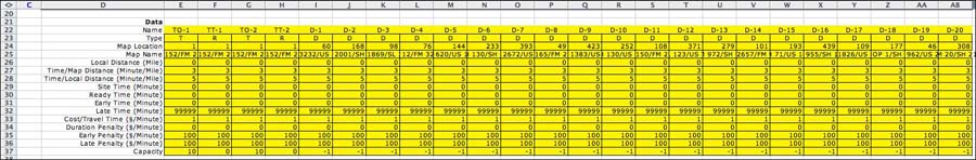
Data Cells |
| |
The sequence of trucks and delivery nodes is described
in row 42. Most of the rows on this form have similarly
named columns on the Data worksheet. The rows 28,
29 and 34 hold parameters related to distance that are provided
by single entries at the top of the data worksheet. The data
cells shown below do not depend on the current sequence. They
are colored yellow to indicate that the cells hold formulas
that link to the data worksheet and remain fixed throughout
the solution process. |
|
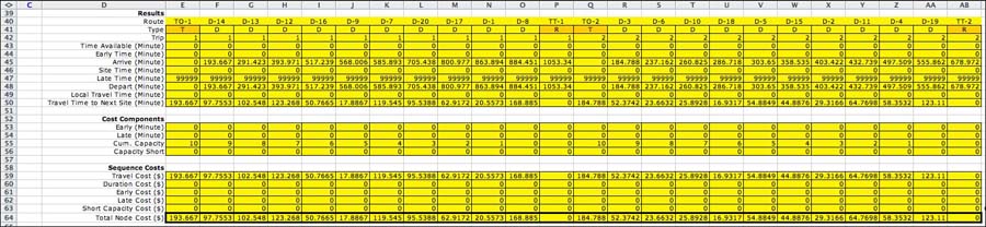
Results Cells |
| |
The results cells starting in row 41 are controlled
by the current sequence. All the cells are colored
yellow to indicate that they contain Excel formulas. The columns
are ordered by the current sequence. The display is dynamic in
that the columns change as the decision variables in row 16
change. For each trial solution, the objective value is computed
from this portion of the worksheet.
The sequence of trucks and delivery
nodes is in row 42. Row 43 identifies the type of the node,
T for origin truck nodes, R for truck terminal nodes, and D
for delivery destinations. The trip row (44) gives an integer
index that indicates the components of the sequence that are
assigned to the various trips. The current example has two
trips representing the routes of the two trucks. The times
available, early times, site times, late times, and local travel
times are transferred by index functions from the data cells.
An arrival time in row 47 is computed as the sum of departure
time of the previous node plus the travel time to the next
node. If this turns out to be earlier than the time available,
the time available becomes the arrival time. The departure
time in row 50 is computed as the arrival time plus the site
time. The travel time to the next node in row 52 is the sum
of: the local travel time from the current node to its map
location, the map travel time between the current node and
the next node, and the local time to the next node.
Row 46 shows the arrival time at each node and row 50 shows
the corresponding departure time. Notice that starting at truck
1, the times increase through the route of truck 1 until the
terminal node for truck 1 is encountered. The
terminal node for truck 1 is immediately followed by the origin
node for truck 2. The arrival time for truck 2 is 480. This
is the beginning of the second trip. The second trip occurs
simultaneously with the first trip. The second trip is completed
by the terminal node for truck 2. |
|
| |
The evaluation of the sequence in terms of
the early and late times and the resource shortages begins
on row 54. Row 55 shows the deliveries that are early, D-4
and D-6. Row 56 shows the deliveries
that are late, D-1 and D-3. Row 57 shows the cumulative capacity
for the sequence. When a new truck is assigned to a trip,
the cumulative capacity for the trip is the capacity of that
truck. As the truck visits delivery nodes, the loads of the
delivery sites decrease the cumulative capacity. A negative
number in this row indicates a shortage. Row 58 reports the
amounts of the shortages. Since the current sequence has no
shortage, the contents of this row are 0.
Rows 61 through 65 numerically evaluate the solution. Row
61 shows the travel costs. The duration costs in row 62 are
computed by multiplying the departure times by the duration
penalties. The example uses 0 as the duration penalties, so
the entries are all 0. The early and late costs multiply
the sum of the early and late amounts by the penalties
for these factors. The contributions of each node to the objective
function are computed in row 66.
All the costs and penalties are accumulated in column T that
is not shown in the figure. The total amount is transferred
to the objective function cell E12 at the top of the worksheet. |
Distance Matrix |
| |
Starting in row 67 is a square matrix holding
the distances between the map locations in the plan. This matrix
addresses data on the distance worksheet. When a table provides
intersite distances and the distance page, the entries to the
matrix on the model page are simple lookup functions addressing
the distance matrix. When the locations are described by the
Cartesian coordinates, the
entries in the model matrix are equations computing the Euclidean
matrix (Pythagorean theorem). When the locations are described
by the geometric coordinates, the
entries in the model matrix are equations computing the Great
Circle distance.
In all cases the matrix does not change with the solution,
so the computation time associated with building the matrix
is experienced only when the matrix is created by the add-in.
This speeds up computation during the solution process. |
|
Location Coordinates |
| |
Row 94 begins a series of rows that compute the
coordinates of the map points in the solution. Geometric coordinates
are used for the map construction of Google Earth. Euclidean
coordinates are used for the Map graphics created by the add-in. |
|
Sequence Optimization |
| |
The Optimize Sequence add-in is used to search
for the optimum sequence. To illustrate the solution process,
we will use the initial solution shown below. The initial
solution is created by clicking the Initial Solution button
on the Results worksheet. The solution is feasible, but it
assigns all the deliveries to the last truck. We will use search
heuristics to find a better solution.
Because it uses heuristic procedures there is no guarantee
that the search will obtain the optimum solution unless all
possible sequences are examined. The algorithm incorporates
several search heuristics that are designed for general sequence
problems but adapted for the routing problem. The process manipulates
the variables in the green cells of row 15 and observes the
resultant objective function in cell E12. |
|
| |
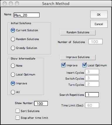
To improve the current solution, click the
Search button at the top of the worksheet. The dialog below
is presented. Click the Improve checkbox at the right
side of the dialog. Also check the local optimum box.
The Improve button on the left of the dialog indicates
that you want to review all the improved solutions encountered
by the process.
|
| |
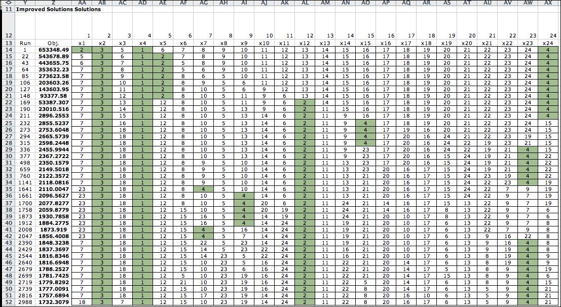
As the search progresses, each solution is placed on the worksheet
and the solution is evaluated by the Excel worksheet functions.
The results of the evaluations are used to direct the search
process.
If the Show Improve button is clicked, the
search process maintains a list of improving solutions. The
figure below shows the results of the search leading to the
example solution. The cells involving truck nodes are highlighted.
These displays are on the Results worksheet. Note
that the objective value at the first run is the initial solution,
subsequent runs have decreasing objective values. The bottom
row is the result of run 2988. It is a local optimum solution
and cannot be improved. |
|
| |
To the right of the next-index solutions,
the associated sequences are also listed. The first few insert
moves divides the deliveries among the two trucks, and the remaining
steps interchange pairs of nodes in the sequence. |
|
| |
Although an acceptable solution
was obtained for this small problem, the search becomes more
difficult as the problem size grows. It also becomes more difficult
as we add complexity to the problem by making the early and
late times restrictive and as more resources are added. The
worksheet evaluation for each solution depends on the size
of the problem. Even one pass through the improvement
process takes a large number of individual evaluations. |
Buttons |
| |
At the top of the page there are
four buttons. The first button displays the Search dialog
shown earlier. The Map button creates the map of the
current solution. This is the same map as the one created by
a similar button on the results page. The buttons on the right
open the unique Results worksheets
corresponding to the Model worksheet.
The yellow cells in the Model worksheet are linked
by formula to the data on the Data worksheet. Any
value changes there are immediately reflect on the model worksheet.
If the number of trucks or deliveries is changed the model
worksheet must be regenerated by the button on the data worksheet.
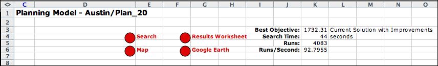
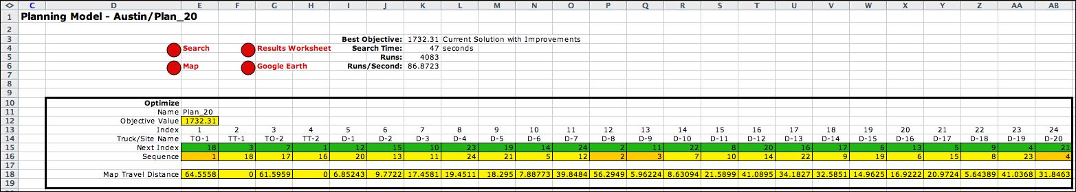
To the right of the buttons are statistics concerning
the computations obtaining the solution. The example required
4083 solution evaluations (called runs). The average number
of runs per second depends on the speed of the computer. The
runs per second decreases as the size of the problem increases.
The total search time is 44 seconds. A local optimum was obtained.
The heuristics used for searching the solution
space are described on the next page. |
| |
|
|