We improve combinatorial solutions by changing one or more variable values in the solution and observe whether the change results in an improvement. With an organized search over some neighborhood of adjacent solutions an initial solution may often be improved. The improvement methods are heuristics in that they do not necessarily find the optimum, but they require many fewer observations than exhaustive enumeration. While exhaustive enumeration methods require exponentially increasing effort to solve problems of increasing size, improvement methods for specified parameters usually require polynomially increasing effort.

We use the integer-nonlinear math programming model shown below. The model shows the solution found with the Excel Solver. Since the continuous version of the objective function is concave, this should be the optimum solution.

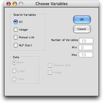
To solve the problem with combinatorial search we choose the Math Program option from the Optimize menu. Select All in the dialog presented.

The only apparent change is the combinatorial form starting in cell U1. Not so obviously, the variables are renamed so the combinatorial search procedures will manipulate the variables in the search for the optimum. The search procedures use the Lower and Upper bounds to limit the range of the search. Although the form shows the Exhaustive search method, that may be changed with the Search command.

Greedy Solution

To improve the solution we choose the Search item from the menu. The various improvement options are illustrated on the dialog below. The Improve checkbox is available for the Random, Current Solution and Greedy Solution methods. Clicking the Improve checkbox initiates the improve option. The two boxes at the lower right set parameters for the improvement. The process will change variables in the solution in a search for a better solution. The box labeled n_change sets the maximum number of variables that will be simultaneously changed. To reduce the number of runs, this number should be set to a small value. The smallest value of 2 is often appropriate. The example uses 3. The second box is the Change. When searching for an improved solution this is the maximum change from the current incumbent solution. The smallest value of 1 is usually sufficient. Larger values will increase the number of runs required. For the example we choose to apply the improvement to the Current Solution because that is the greedy solution.

For the general or range model the improvement process is as follows. First the greedy enumeration method is applied to the current solution. Then we perform the 2-change method on the current solution. This means that every pair of variables is selected in turn and the values of the variables are caused to vary between (+,-) the maximum change from the current incumbent solution. Whenever a solution is encountered that has a better objective value than the incumbent, the solution becomes the incumbent solution. The 2-change procedure is repeated until there is no improvement. For a particular pair of variables, only solutions that are different for both variables are considered.

If the n-change value is greater than 2, the program next performs the 3-change procedure. Here all combinations of three variables are considered in turn and all variables are allowed to assume values between (+,-) the maximum change from the current incumbent solution. For a particular set of three variables, only solutions that are different for all variables are considered. The 3-change procedure is repeated if any variable values are changed. The process repeats for 4-change, 5-change, etc if called for by the dialog. The results for the example are shown below. During improvement, only improving solutions are shown in the list because the process may evaluate the same solution many times.

The improvement process finds a solution with value 146.42. This is not the optimum but it is much improved from the greedy solution. In the summary of runs "Imp." indicates the number of objective evaluations required to perform the improvement process.

Improving Random Solutions