To illustrate the Fibonacci enumeration and compare it with exhaustive enumeration we use a forecasting example as in the figure below. The example was constructed with the Forecasting add-in. It uses a simulated time series with random step increases and decreases in the mean value. This example is simulated for 200 periods beyond a 20 period warm-up interval. The forecast of interest is 2 periods beyond the current period. For example the forecast at time 2 is based on the estimate of the time series mean at time 0. Note that if you are running the example from the demo worksheet the Forecasting add-in must be installed. To assure that the formulas on the worksheet are linked to the add-in, choose the Relink command from the Forecast menu.

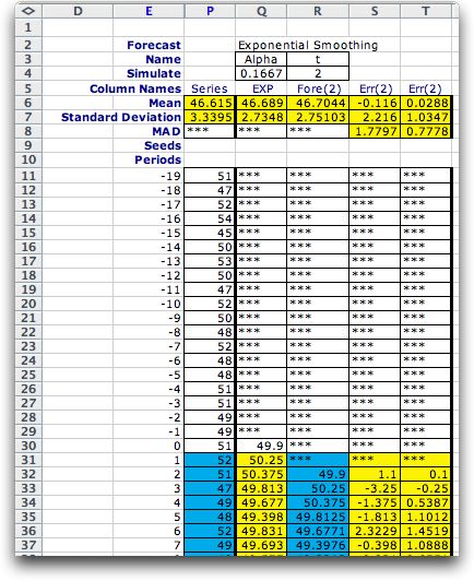
The exponential smoothing method requires a single continuous parameter alpha that ranges from 0 to 1. To convert the search for an optimum alpha to a discrete space we use a transformation common in forecasting practice:

alpha = 2/(m + 1) where m takes on integer values.

The value of alpha used for the figure below is computed with m = 11, the value that turns out to be optimum. We use the Mean Average Deviation (MAD) computed in cell S8 as the criterion for optimality. We are to find the value of m that minimizes the MAD. In practice such a result is useful because it suggests the best parameter for forecasting a particular time series.

The example has a single decision variable that ranges from 1 to 20. To create the form we choose the Add Form option from the menu and set the parameters as below.

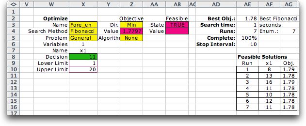
After the form is constructed we choose the Fibonacci search method.

Fibonacci search is based on the Fibonacci sequence. The first two Fibonacci numbers in the sequence are both 1. All others are obtained by adding the previous two numbers in the sequence. The first ten Fibonacci numbers are shown below.

This search method is valid if the objective function is unimodal. For a minimization this means that is it has no more than one change in direction as the variable is increased. We will see that for this example the MAD when m =1 is 2.2367. As m increases the MAD decreases until its value is 1.7797 at m = 11. Thereafter the MAD increases as m increases. Thus the MAD is unimodal in this case.

With N observations, this search method can find the optimum integer value in an interval of length F(N + 1), where F(N) is the Nth number in the Fibonacci sequence.

For the example we are searching the integers 1 through 20. We take the initial interval as 0 to 21 since the search procedure does not enumerate the end points. We note that F(7) = 21, so 6 observations are necessary. The results are shown in the table below. The observations are placed according to the numbers in the sequence. To search the interval of 21, the first two observations are at 8 and 13. The value at 13 is the smaller, so the optimum cannot lie below 8. The interval is now (8, 21) and the two observations are at 13 and 16. Since the objective at 13 is already known, only the value at 16 must be computed. Since the value at 16 is greater than at 13, the interval that holds the optimum must be (8, 16). To further reduce the interval, an observation is placed at 11. Since this value is smaller than the value at 13, the interval is now (8, 13). The next observation is at 10. Since the objective at 10 is greater than at 11, the interval is now (10, 13). The last observation is at 12. Again this value is greater than at 11, so the interval is reduced to (10, 12). Only the observation at 11 is within this interval and the optimum has been discovered. At termination, the optimum value (11) is repeated and appears in the list as run 7.

The search process requires that the cell holding the value of alpha, Q4, be linked to the decision variable at X8. This is implemented for the example by placing the following formula in Q4.

= 2/(X8 + 1)

Note that the formula linking the combinatorial variable to the model variable need not be a simple assignment (=X8), but can be an arbitrary function of the combinatorial variable.

Similarly, the objective for the problem must be placed in cell Z4. We do this by placing the following formula in cell Z4.

= S8

Cell S8 holds the value of the MAD for the simulated time series. The process sequentially places the six values of the decision variable in cell X8 and the value of the MAD is computed for each decision alternative with the formulas on the worksheet. The code of the add-in controls the search process.

We do not use the feasibility cells, AB3 and AB4, since there are no logical conditions that restrict feasibility other than the limits on the variable. It is important that the default value TRUE remain in cell AB3 since all solutions generated are feasible.

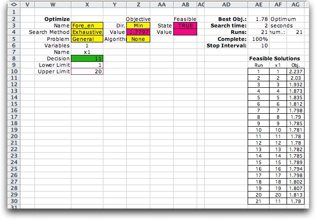
For comparison, we show the exhaustive enumeration below. Exhaustive enumeration requires 20 observations. The feature of unimodality can be seen from the unsorted list of results in column AR. Since the function is unimodal, both methods find the optimum solution. Run 21 recomputes the optimal solution.

We must observe that the MAD for a finite forecast is not always a unimodal function of the parameter m. It is often the case that for simulated data the objective will be "bumpy". The expected value of the MAD may be a unimodal function of the parameter, but the average of a simulated realization may not. In these cases the Fibonacci method must be viewed as a heuristic. We use it to reduce the number of observations required to obtain a solution, but accept the fact that the method will not always yield the optimum solution.

More than one Decision Variable

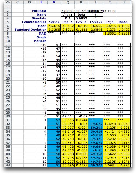
We also allow the Fibonacci method to be used with more than one decision variable. We use as an example the same time series as before, but now we forecast with the exponential smoothing with trend method. This method estimates a constant term and a linear trend coefficient. Forecasts are made with a linear projection. In the figure below the constant term is in the column labeled Exp. a, and the linear coefficient is in the column labeled Exp. b. The forecast interval is 2 and the forecasted values are in the column labeled Fore(2). To illustrate, we compute the forecast in period 2 from the constant and linear terms shown for period 0 (row 30).

F(2) = a(0) + 2*b(0) = 49.7143 + 2*(-0.0195) = 49.6742

The error shown in Err(2) is the difference between the observed value at period 2, 51, and the forecast.

The values of a(t) and b(t) depend on the data of the previous periods based on the forecasting method. This method has two parameters alpha and beta. We would like to choose these two parameters to minimize the MAD, the mean absolute forecast error, computed in cell T8. The values shown in cells Q4 and R4 are the best values determined by the enumeration.

To find the optimum parameters, we construct the form below using the Add Form menu command with two decision variables. The forecasting parameters in Q4 and R4 are linked to the variables in Y8 and Z8 with the formulas:

alpha = 2/(Y8 + 1), beta = 2/(Z8 + 1)

The objective value in AA4 is linked to the MAD with the formula:

value = T8

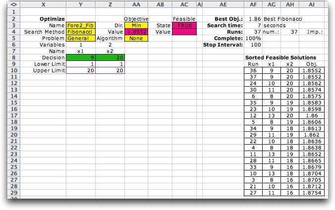
With more than one decision variable, the Fibonacci method finds the optimum solution sequentially. With the range 1 to 20, each Fibonacci search requires six observations. The variables are considered from left to right. For each value considered for x1, six observations are made to obtain the optimum value for x2 and the associated optimum objective value. Since there are 6 values for x1, a total of 6*6 or 36 observations are required to find the best solution.

The results are shown below. We also show the best 20 solutions found during the search. It is not surprising that the value for x2 (m for beta) is large. The simulated time series only has step changes, not trends, so the best value of beta should be as small as possible (x2 should be as large as possible).

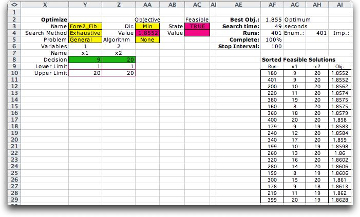
For comparison we show the solution obtained by exhaustive enumeration. Exhaustive enumeration requires 20*20 or 400 observations. As expected the time required to obtain the optimum is greater. For the example, exhaustive enumeration yields the same solution as Fibonacci search. We see new solutions among the top 20 solutions because exhaustive enumeration evaluates so many more solutions than the Fibonacci method.

Discrete Fibonacci search only works reliably when there is a single decision variable and the objective function is unimodal with respect to that decision variable. In a multivariable problem, there is no guarantee that an optimum solution will be found. We provide this option because many fewer solutions need be evaluated than for exhaustive enumeration when the range for the decision variables is large. For many problems the results will be nearly optimal.

As for exhaustive enumeration, Fibonacci search requires an exponentially increasing number of observations as the number of variables is increased. When only two values for each decision variable are feasible (say 0 and 1), the two methods require the same number of observations. Only when the range is greater than 3 will the Fibonacci method result in a reduction. When the range is large, the reduction in the number of observations is considerable.

Feasibility

In this example there were no additional conditions limiting feasibility. Thus cells AC3 and AC4 play no role for the example. In other situations, the State cell (AC3) may contain a Boolean expression indicating by the state TRUE or FALSE whether the solution is feasible or not. For the Fibonacci method we must also provide a measure of infeasibility in the Value cell. This is a formula that returns positive values for infeasible solutions. Although a 0 value for a feasible solution is desirable, the program neglects the value for feasible solutions.

For infeasible solutions a term is added to the objective value that is:

infeasibility measure squared multiplied by the infeasibility weight.

The infeasibility weight is entered in the Search dialog. Its default value is 10. Since the algorithm treats all problems as minimizations, solutions far from feasibility will be penalized with very large objective values. This forces the Fibonacci search to select solutions that are feasible rather than infeasible. Also if the method compares two solutions that are both infeasible, the procedure will judge the one with the least infeasibility as the better one.