One option of the Math Programming add-in is to create a linear network flow model. By selecting Math Program from the Optimize menu when a network model is on the active worksheet, the Optimize add-in constructs a form for discrete variables that can interact with the linear network model. When all the variables are specified as the combinatorial variables in the dialog, the network flow variables are manipulated directly by the search process. A more interesting case is illustrated here in which the combinatorial problem involves a selection of arcs that are to be excluded or included in the network. In this example, we manually link the combinatorial variables to the network model. For this example, three add-ins must be installed, the Math Programming add-in, the Network Solver add-in and the Optimize add-in.

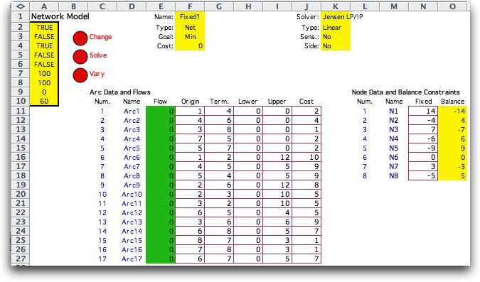
Consider a telecommunications network in which traffic flows between various origins and destinations. The figure shows a case with three source nodes S = {1, 3, 7}, four destination nodes D = {2, 4, 5, 8}, and one transshipment node T = {6}. The arcs drawn with solid lines represent existing communication links while those drawn with dashed lines are proposed links. The complete set of arcs is denoted by A = {1,…,17}.

Associated with each link is an upper bound on flow and a unit flow cost shown as the two numbers on each arc. If one of the proposed links is constructed, it will have the capacity and cost indicated on the arc. Let A' = { 1,…,5} be the set of proposed links with corresponding construction costs f1 = 8, f2 = 6, f3 = 9, f4 = 7 and f5 = 7. These costs are independent of size. The problem is to determine which links to build, if any, and how much traffic to put on each link in the network so that the sum of the flow costs and construction costs is minimized. For a solution to be feasible, it must satisfy flow balance at each node and arc flows must stay within the arc capacities.

The model constructed by the Math Programming add-in is below. The first 5 arcs are those shown as dotted in the figure. The model has all the arcs open. The solution with all arc flows at 0 is not feasible since it violates the node balance constraints.

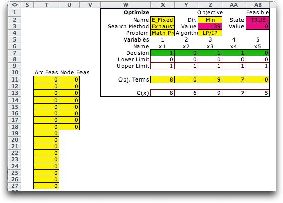
We choose Math Program from the Optimize menu to construct an combinatorial form on the worksheet. There is a variable for each fixed charge arc.

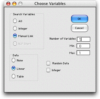
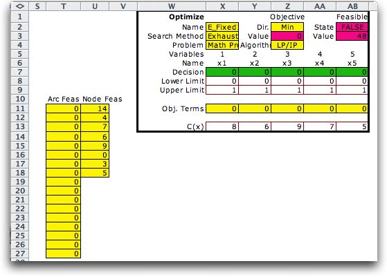
The form is placed to the right of the network model. The two arrays in columns T and U measure the infeasibility of the current flow solution. With all 0 arc flows, the flows satisfy the arc capacity constraints, but the balance at the nodes is not feasible. Infeasibility is indicated by a positive numbers in the feasibility arrays. Formulas are placed in cells AB2 and AB3 to indicate feasibility of the flow solution. The data form in row 13 holds the fixed costs, and the contribution to the objective is computed in row 11 and totaled with the network cost in cell Z3. The requisite formulas in the yellow cells are inserted by the add-in.

It is necessarily to automatically link the network model with the combinatorial variables representing the fixed charges. We do this by placing formulas in the upper bound column for each of the first five arcs. For example in cell I9 we insert the formula:

=10*X7

Here X7 holds the value of y1. When X7 is 1, the bound on flow is 10 and the arc is included in the model. When X7 is 0 the bound on flow is 0 and the arc is excluded.

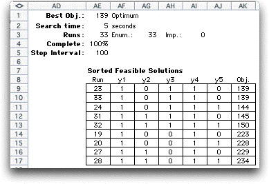
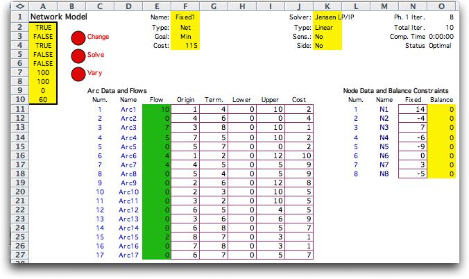
We have chosen to exhaustively enumerate the 32 solutions for the 5 combinatorial variables and the optimum result is shown below. It is optimal to open arcs 1, 3 and 4. The value in Z3 is the total of the fixed costs and the cost of the network flow solution.

This problem could have been solved as a mixed-integer-linear program since adjusting the upper bounds on an arc can be implemented with a linear constraint. The adjusted network model has side constraints and integer variables and it is no longer possible to solve the embedded network problem with a network solver.

The models shown here are much more intuitive and easy to implement in Excel. The resulting combinatorial problem is easy to solve by enumeration for this small case and the network flow models are solved with the Network Solver. For larger problems, exhaustive enumeration would not be possible and one of the approximate solution methods would have to be used.

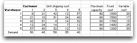
When a transportation model constructed by the Math Programming add-in is on the worksheet when Math Program is selected from the Optimize menu, a form is created that allows manual linking of combinatorial variables to elements of the transportation model. As an illustration we consider a small warehouse location problem with data shown below. There are five customers and five locations where warehouses can be located. The customer demand must be served, but all the warehouses need not be constructed. Unit shipping costs between the customers and the potential warehouse locations are given. The fixed and variable costs associated with each warehouse are in the table at the right. An open warehouse can serve up to 80 units of demand.

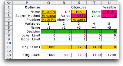
Given the set of open warehouses, the optimum shipping pattern can be determined by a linear transportation model. We model the combinatorial problem of selecting the warehouses separately from the problem of distributing the product. The combinatorial form with the optimum solution is shown below. It is optimum to open warehouses at locations 1, 3 and 4.

The transportation model is below. The Max. shipments shown in column J are determined by equations that link to the combinatorial warehouse decisions. The add-in adds the feasibility formulas in column M and row 18.

The results of the exhaustive enumeration are shown below. Only feasible solutions are shown.