The Math Programming add-in creates a structure that is useful for specifying the objective function and constraints of an algebraic optimization model. An example is shown below. The model has a nonlinear objective with separable linear and quadratic terms. The coefficients of the linear terms are in row 12. Row 13 holds the square of each variable and row 14 holds the quadratic coefficients. This objective is a convex function.

Even without the integrality requirement the model shown is difficult to solve. The objective is to maximize a convex function in a linearly constrained region. For the continuous problem (dropping integrality) there are several local maxima at the extreme points of the feasible region. The solution obtained with the Excel Solver depends on the initial solution. For example when the initial solution is set to all 0's, the Solver terminates at the solution with all 0's, however, this is not the global maximum. We will use exhaustive enumeration to solve the problem.

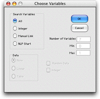
To treat the math programming model as a combinatorial problem choose Math Program from the Optimize menu. The dialog below is presented.

The buttons in the Search Variables region of the dialog select the variables to be used for the combinatorial optimization. For this example we choose the All button. This means that all the model variables will be varied in the search for the optimum. We illustrate the other choices later.

The worksheet is modified in several ways by the add-in. The cells that represent the model variables, Values and the Lower and Upper Bounds, receive new names so that they also become the combinatorial variables and their limits. Thus the range H8:N8 holds both the math programming variables and the combinatorial variables, so it is unnecessary to manually link them. Similarly, cell F4 is assigned a new name so it represents both the model objective function and the combinatorial objective function, again removing the requirement to manually link the two cells.

Formulas are added to the right of the model (column O for this case) that compute the values of the slack variables for the constraints. In the next column (P) formulas are included that evaluate as positive quantities for violated constraints and 0 for satisfied constraints. A value in column P shows the amount by which a constraint is violated. Since the current solution is feasible (all 0's) and all the constraints are satisfied, column P holds all 0's. The figure below shows the added columns.

Exhaustive Enumeration

We choose to solve the problem with exhaustive enumeration. The remainder of the combinatorial cells constructed by the add-in are shown below after exhaustive enumeration is complete. Cell U3 holds the sum of the numbers in the range P17:P21, and cell U2 returns TRUE if the sum is 0 and FALSE if the sum is positive. Thus cell U2 indicates whether a given solution is feasible. Selecting the Search command from the menu initiates exhaustive enumeration. The optimum solution has x6 = x7 = 2, and all others equal to 0.

The seach process evaluates each of the 2188 solutions allowed by the lower and upper bounds of the variables. During the process, the program collects the 20 best feasible solutions and presents them starting in column W. The optimum appears at the top of the sorted list.

Any of the search methods can be applied to the model by simply selecting the method in the search dialog. Of course options such as greedy search or random search may yield a solution in fewer iterations, but the solution found may not be optimum. Note that we are using combinatorial search rather than math programming to solve the problem. The math programming add-in simply provides a convenient structure on which to define the model.

To perform a greedy approach, select Greedy from the Search dialog.

A partial list of the solutions investigated by the greedy approach is shown below. The list presents the solutions in the order generated. Only variations that provide improvement and are feasible are shown in the list. Although 37 solutions were examined only 25 are shown. Each iteration begins from the incumbent from the previous iteration. The first incumbent is the initial solution with all zeros. The first set of iterations examines all solutions obtained by changing each variable by 1 unit. Only positive variations are attempted because the variables are bounded from below by 0. The best solution obtained is:

x = (0,0,0,0,0,1,0), z = 4.9

Iteration 2 starts from this solution and examines all solutions obtained by unit changes of each variable. The best for iteration 2 is:

x = (0,0,0,0,0,2,0), z = 21.8

In a similar manner, iteration 3 starts from the best solution of iteration 2 and finds the improved solution:

x = (0,0,0,0,1,2,0), z = 23.8

Iteration 4 starts from the best solution of iteration 3 and finds the improved solution:

x = (0,0,0,0,2,2,0), z = 31.8

Iteration 5 cannot improve on this solution and the greedy method terminates. Run 37 simply replaces the current solution with the best of the 36 previous runs.

At each iteration tries to improve the best of the previous iteration. When an improving move cannot be found the methods stops.

The best solution found happens to be the optimum determined by exhaustive enumeration, however the greedy process only requires 37 solutions evaluations while exhaustive enumeration required over 2000. Of course this fortunate result cannot be guaranteed. The number of solutions evaluated depends on the parameters of the problem, but the effort grows polynomially with the size of the problem.

We have illustrated the greedy solution applied to the math programming model. The method only uses the objective value to select the improving variable. Feasibility is considered by adding a penalty for solutions that violate the constraints. The values of the constraint coefficients for the variables do not affect the choice of the improving variable.

A solution obtained with greedy enumeration can be improved by performing the improvement procedures described on the next page.