The add-in places the TSP form on the worksheet with the upper-left corner located at the cell specified in the dialog. The data for a 7 city problem is shown below in the range labeled C(To, From). With the Euclidian option chosen for the example, the city locations are placed in columns J and K. The integer parts of the Euclidean distance comprise the table. City 1 starting city is identified as x1. x1-ret. represents the same city when the tour is complete. Note that the locations for city 1 and city 8 are the same.

The decisions for the TSP, in row 7, indicate for each city the next city in the sequence. The sequence associated with the decisions is computed and shown in row 8. The default initial tour starts at city 1, passes to city 2 and so on until city 8 is reached. The first and last cities are connected by a 0 length link. The program uses the Excel Index function in row 10 to compute the distance traveled from each city, and the total distance is computed in cell D3. Although the Euclidean distances are symmetric, this feature is not required by the solution methods.

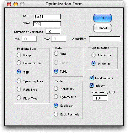
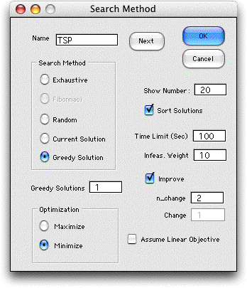
To solve the problem we choose Search from the Optimize menu. We have chosen to exhaustive enumerate all solutions.

On pressing OK, the add-in computes the number of solutions that will be enumerated and presents the option whether to continue. The add-in generates only valid tours.

For a problem not much larger than this one, the number of solutions becomes exorbitant and one should choose not to continue. For example, the ten city problem has 362,880 tours. Although evaluating this number of solutions is not impossible, the serious user should look elsewhere for more efficient methods. The add-in will not begin problems with more than 1,000,000 solutions.

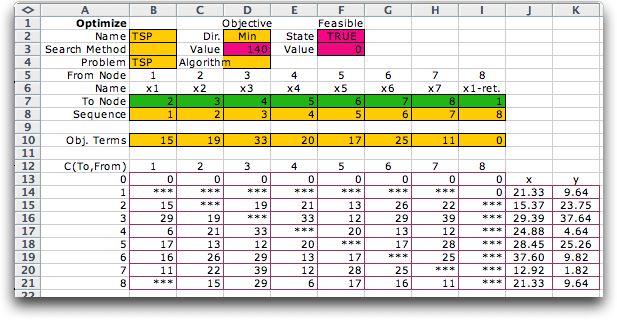
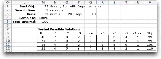
During the solution process, the add-in generates and evaluates all valid tours. The best 19 solutions are placed to the right of the data. The optimum solution is evaluated twice and is shown at the top of this sorted list. The solution shows the city that follows each city in the sequence. Thus x1 = 7 means that city 7 follows city 1. The remainder of the tour is derived from the solution.

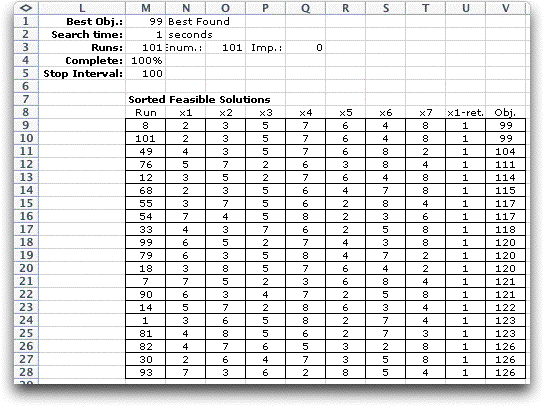
Optimum Tour = (1, 7, 4, 6, 5, 3, 2, 8, 1)

The second solution has the same length (99). In a symmetric problem there will always be at least two optimum solutions. Based on the second solution the alternative optimum is

Optimum Tour = (1, 2, 3, 5, 6, 4, 7, 8 ,1)

The tours follow the same sequence but in opposite directions.

During the enumeration process each tour is placed on the worksheet in row 7 of the data form and the add-in uses the Excel computations to evaluate the solution. This method can be adapted to a variety of sequencing problems other than the TSP by changing the formulas that compute the objective function. Although we have not used the Feasibility cells (F2 and F3) for the TSP, these cells might be useful for other problems that have feasibility conditions not otherwise modeled.

Heuristic Methods

Of course, exhaustive enumeration is possible only for TSP's of small dimensions. The add-in provides heuristic methods to search for the optimal solution for larger problems. One possibility is to generate tours at random. The sorted list below shows the results obtained with 100 random tours. It happens that the optimum solution was discovered for this small example.

Another option is to use a greedy approach to find a solution. The program uses the nearest neighbor approximation. The tour starts at city 1, the next city is the one nearest to city 1 according to the distance measure. This is city 4. The closest to city 4, not yet visited is city 7. The tour construction process continues by adding the closest city not yet visited to the tour. This myopic approach fails to find an optimum tour for the example. In general the process does not guarantee the optimum and there are examples where the result is far from optimum.

The add-in also provides an improvement method that operates on a complete tour. The method uses the n-change parameter with the smallest value of n-change equal to 2. The dialog below shows the option of generating a greedy solution and implementing the 2-change improvement.

The program considers each pair of tour indices and evaluates the effect of switching the two cities at these indices. If the tour length is reduced (improved), the switch is made. The process continues until no improving switches are found. The table below shows the result when the 2-change improvement is applied to the greedy solution. Following table from the bottom up shows the improving decisions and the best solution found is at the top. Two changes were made and the final solution happens to be the optimum. Only improving solutions are shown during the improvement process.

Row 3 of the worksheet shows the number of feasible runs required for the process. The number labeled Enum is the number of evaluations made during the greedy process. In this case 22 evaluations of the worksheet leads to the greedy solution. The number labeled Imp is the number of evaluations of switched cities during the improvement process. In this case, three passes through the process were required with 15 evaluations for each. The first two passes resulted in improved solutions. The process stopped when no improvements were made in the third pass. It is impossible to estimate accurately the number of passes for an improvement process since the number is problem dependent. The number of improvement evaluations is increased by 1 for each pass because the add-in evaluates the incumbent solution prior to each pass.

The add-in allows larger values of n-change. With a value of 3 all interchanges of three cities are considered. As n-change becomes larger the number of improvement evaluations increases considerably but the final result may be closer to optimum. A value of n-change equal to one fewer than the number of cities is equivalent to exhaustive enumeration.

The improvement process can be applied to the current solution on the worksheet, the results of the greedy procedure, or to each of a set number of randomly generated solutions. The latter case is often a good heuristic since it combines the impact of random generation and improvement. Only a few random solutions should be generated with this option because the number of random solutions multiplies the number of improvement evaluations.

Using heuristics there is no limit to the size of the TSP except the dimensions of the Excel worksheet. A feature of the n-change heuristic is that for a specified number of initial solutions, the number of improvement runs in each pass grows algebraically with the number of cities rather than exponentially. More examples of the improvement techniques applied to the TSP can be found on the next page. With the Combinatorics add-in we attempt a 48 city problem. That size problem is too large for the generic approach of the Optimize add-in.