|
|
 |
Optimize |
 |
-Permutations |
|
Several problems are solved by finding an optimum permutation
of the first n integers. As an example consider the
simple assignment problem. There are n tasks and n
machines. A cost is specified for completing each task with
each machine. The problem is to assign one task to each machine
so that all tasks are completed with the smallest total cost.
This is a combinatorial problem whose solution is described
by a permutation of n integers. For a seven task problem
one solution is given by the permutation: (1, 2, 3, 4, 5, 6,
7). This implies assigning task 1 to machine 1, task 2 to machine
2 and so on. Every permutation describes an assignment.
The linear assignment problem just described is one of the
simplest of the combinatorial problems and can be solved with
linear programming as well as with several special purpose algorithms.
Here we formulate and solve the problem as a combinatorial search
problem. Although this is a poor choice from a computational
point of view, it serves to illustrate the features of the Optimize
add-in for permutation problems. There are a number of problems
whose solution is a permutation that that are not so easy to
solve including the quadratic assignment
problem and the facility
location problem. These problems are solved in the Combinatorial
add-in and the Layout add-in with procedures that call
the permutation option of this Optimize add-in.
To create a permutation model choose Add Form from
the Optimize menu. In the dialog click the Permutation
button and enter the number of variables into the appropriate
field.
With the data table box checked a square matrix is included
to hold the cost of the assignments. With the data table, the
problem definition is complete and the model may be solved directly.
Without the data table, the user must construct the formulas
for the objective function and feasibility conditions. |
| |
|
| |
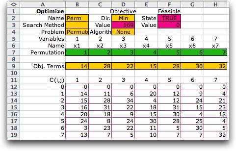
The add-in places
the permutation form on the worksheet with the upper-left corner
located at the cell specified in the dialog. The data for a
7 task-machine assignment problem is shown below in the range
labeled Obj. Coef. The table shown holds randomly generated
data. Row 0 is used by the program and should not be changed.
We arbitrarily call the rows tasks and the columns machines.
The decisions in row 7 are a permutation that represents an
assignment. The initial solution assigns task 1 to machine 1,
task 2 to machine 2 and so on. The program uses the Excel Index
function in row 9 to return the cost for each machine,
and the total cost is computed in cell D3.
Note that this combinatorial representation of the assignment
problem is much different than the representation used for linear
programming models. For the latter, the variables take on the
values 0 and 1 where x(i,j) = 1 if task i is assigned to machine
j and 0 otherwise. The LP model has a constraint for each task
and each machine that assures that every task is performed exactly
once and every machine is used exactly once. In the combinatorial
model the values are integers that range from 1 to the number
of tasks. The objective function is not linear since it uses
the Excel Index function. This model is concise with only 7
variables and no constraints while the linear programming model
has 49 variables and 14 constraints (one is redundant).
In the present case one pays for the combinatorial simplicity
with computational tractability. While the LP model is easy
to solve, the combinatorial model requires an exponential optimization
procedure or approximate solutions. |
|
| |
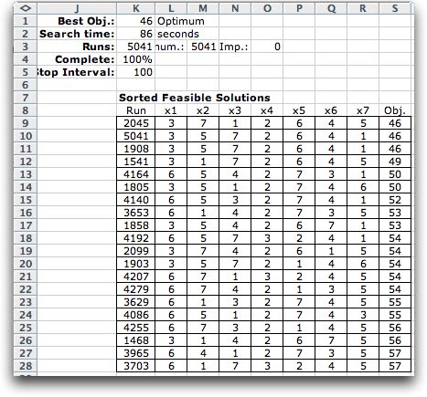
Solving the combinatorial model by exhaustive
enumeration requires that 5041 permutations be evaluated. Only
permutations are generated and each is placed in row 7 of the
combinatorial form. The worksheet functions compute the value
of each solution and the add-in keeps track of the best 20 found.
The results for the example are below. |
|
| |
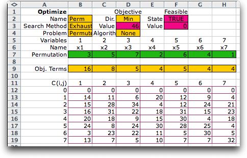
The optimum permutation is placed
on the combinatorial form. |
| |
| |
This method can be adapted to a
variety of permutation problems other than the assignment problem
by changing the formulas that compute the objective function.
Whatever the objective, the results must be a function of the
permutation and be computed in cell D3. Although we have not
used the Feasibility cells (F2 and F3) for the assignment,
these cells might be useful for other problems that have feasibility
conditions not otherwise modeled. |
Random Search |
| |
Of course, exhaustive enumeration
is possible only for small dimensions. The add-in provides heuristic
methods to search for the optimal solution for larger problems.
One method is to generate permutations at random. By clicking
the Improvement button on the Search dialog,
each randomly generated solution will be subjected to the improvement
procedure. |
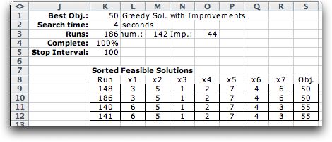
Greedy Solution |
| |
Another option is to use a greedy
approach to find a solution. This is a constructive procedure
that adds one machine-task assignment at a time. When a data
table is present, the program computes the difference between
the smallest number in a column and the next smallest number.
The first assignment is made in the column with the greatest
difference. The row with the smallest cost is chosen for the
assignment. Subsequent assignments compute column differences
and make assignments from rows and columns that have not already
been used. The table below shows the results of the greedy assignment
followed by an improvement step. The greedy solution is obtained
in run 140. The improved solution was obtained in run 148 by
switching the assignments for x1 and x7. The improved result
is not the optimum.
The greedy approach takes a number of objective
evaluations that involve incomplete assignments. The greedy
approach only finds a feasible solution at the last step.
When the data table is not present, the objective
computation must be provided by the user. Every observation
requires an evaluation of the worksheet and the greedy approach
may take quite a few evaluations, but the effort generally takes
a small time compared to the other search approaches.
The greedy approach often encounters tie values
during the construction process. When this occurs the assignment
pair is chosen at random. When ties are present, several calls
for greedy search may yield different solutions. A box on the
search dialog allows the program to perform several greedy searches
sequentially. |
Improvement |
| |
Given a permutation, the values
for any set of variables may be switched and the result will
still be a permutation. The program uses an n-change switching
approach in the search for improvements, where n-change is at
least 2. With n-change equal to 2, all pairs of variables are
considered and the values of the variables are temporarily switched.
The resulting permutation is evaluated and if the objective
value is improved the two values are switched for the subsequent
steps of the process.
The add-in allows larger values of n-change. With a value of
3 all interchanges of three variables are considered. As n-change
becomes larger the number of improvement evaluations increases
considerably but the final result may be closer to optimum.
A value of n-change equal to one fewer than the number of tasks
is equivalent to exhaustive enumeration.
For n-change greater than 2, the process starts by investigating
all possible 2-variable switches. The process continues until
a complete pass through the entire set results in no improvement.
Then the process considers all 3-variable switches until no
improvement is observed. The process continues to consider changes
until the specified n-change value is reached. For any number
of switches we require that all switched positions be changed.
This assures that k-variable switches do not repeat switches
already considered with fewer than k variables.
The improvement process can be applied to the
current solution on the worksheet, the results of the greedy
procedure, or to each of a set number of randomly generated
solutions. The latter case is often a good heuristic since it
combines the impact of random generation and improvement. Only
a few random solutions should be generated with this option
because the number of random solutions multiplies the number
of improvement evaluations. |
| |
|
|