The add-in allows the solution of mixed-integer programming models with the combinatorial methods. If the integer variables affect the model in a linear fashion, the model is then a mixed-integer-linear model and can be solved using branch and bound implemented by either the Excel Solver or the Jensen LP/IP add-in. The search approach described here also handles problems where the integer variables affect the objective and constraints in a nonlinear or combinatorial fashion. This is an interesting and valuable feature since many practical situations have these characteristics.

The add-in solves problems by searching over the combinatorial variables. The remaining variables must define a linear programming model since their values will be found using the linear programming simplex technique. The simplex technique is implemented in the Jensen LP/IP add-in. Of course, the LP/IP add-in must be installed for the methods to work.

For convenience we illustrate the add-in with the mixed-integer-linear model shown below. The first three variables are required to be integer as indicated by the I's preceding the indices in row 6.

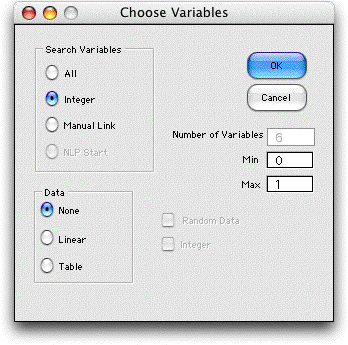
To construct the combinatorial form we select Math Program from the Optimize menu. The dialog below is presented.

Here we choose the Integer option. The combinatorial form shown below is constructed for the three variables identified on the model as integer.

The Objective value cell (T3) is linked to the objective function of the model. The feasibility State (cell V2) and Value (cell V3) are determined by the slack variables for the model. These cells are automatically filled by the add-in.

On the model, the lower bounds and upper bounds of the integer variables are linked to the decisions in the combinatorial form. The linking equations are shown for X1 in the figure below. The upper and lower bounds of the decision variables are set equal to the combinatorial variables. As the search proceeds the math programming model is reduced to an LP in three continuous variables. The add-in creates columns to compute the slack and feasibility values for the constraints. The feasibility values are positive for infeasible solutions.

Note that we have handled the integer variables by combinatorial methods while using the LP simplex method to solve the continuous variables. The add-in enumerated each integer solution and placed it on the combinatorial form. The Excel formulas transferred the solution to the lower and upper bound rows of the math programming form and the Jensen LP/IP add-in solved the resulting LP. Although we have illustrated this feature on a simple problem that could have been solved with a single call to the LP/IP algorithm, this combination of combinatorial search and linear programming can be a powerful solution tool.

We have used exhaustive enumeration for this example, but all of the search methods previously described are available. For larger problems, we may not be able to find the optimum, but we may be able to find a good heuristic solution with the other approximate methods.

The third option for math programming enumeration is to manually establish the links from the enumeration variables to the linear programming model. For this example, we consider the same model, but we do not require any of the variables to be integer. The model showing the LP solution with the original constraints is below.

We want to modify the model to allow the purchase of greater values of the RHS for the constraints. Of course if the RHS values are increased, the optimal solution will most likely have a corresponding increase in the optimal objective function. We assume an individual constraint RHS can be increased by 12 units for a cost of $7.

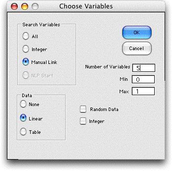
We choose Math Program from the Optimize menu and click the Manual Link button. We enter 5 as the number of variables, one for each constraint. We also click the Linear button to create a data array for linear coefficients.

The combinatorial form is below. The data table includes a row for the linear contribute of the combinatorial variables. The objective function of the combinatorial form is the sum of this linear contribution and the solution of the LP. We have manually modified the RHS vector of the math programming model to refer to the enumeration variables. For example in cell F15 we place the formula:

= 35 + 12*R7

When R7 is 0, the RHS for the first constraint is 35. When R7 is 1, the RHS is 47. The other RHS values are similarly replaced. As each alternative for the combinatorial variables is considered, the RHS vector is changed and the corresponding LP is solved with the LP/IP add-in. With the Manual option it is necessary to link the combinatorial form with the math programming form manually, but any relationship is allowed.

The results of the enumeration are shown below. The list shows the top 20 solutions. The optimum adds extra resources to constraints 3 and 4.

The LP solution with an extra 12 units for constraints 3 and 4 is shown below. During the course of the enumeration 33 separate LP problems were solved. The one shown is for the optimum solution.

When a math programming model is on the active worksheet, selecting Math Programming from the Optimize menu allows all or part of the model to be solved with combinatorial methods. Of course when the model is naturally a linear-integer or linear-mixed integer model, it is more readily solved directly by the Excel Solver or the Jensen LP/IP Solver. There are situations however, when it is necessary or convenient to treat part of the problem with combinatorial methods. For these situations the add-in will be useful.

The same facility is available for network flow and transportation models. This is described on the next page.