|
|
 |
Optimize |
 |
-
Combinatorial Form |
| |
| |
To illustrate the process of adding
an optimization form we use the Job Shop queuing network example
shown below. The example is fully described in the section on
the Queues add-in.
The Queues add-in also has a new menu
item that provides for constrained optimization of queuing
models. The network consists of six stations labeled A through
F. The system shown below uses the fewest number of servers
that yield a stable result with a total of 15 servers used.
We want to investigate the effects of adding more servers. The
measure of interest is the mean time in the system
computed in cell J9. Of course this time can be reduced to its
minimum by adding an unlimited number of servers, but here we
limit the total number of servers to 20, five more than the
minimum. The number in cell J9 is a complicated function of
the number of servers involving several formulas. Some user-defined
functions provided by the Queues add-in
are used in the computation, so Queues add-in
must be installed to build and solve this model. If you open
this model from the Optimize demonstration file, you must choose
the Relink command from the Queues menu before
proceeding. |
|
| |
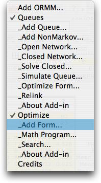 |
To begin the analysis, we choose the Add
Form command from the menu. The Queues add-in
commands appear in the list because that add-in is installed
for the example. The dialog below is presented.
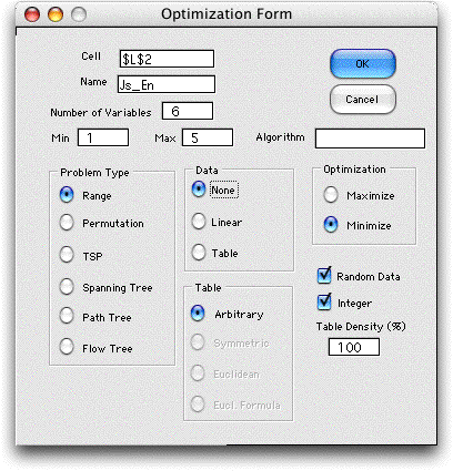
The form must be placed so it does not disturb
the cells describing the queuing network. Cell L2 is to
the right of the model. The Name is used by the
add-in to provide Excel range names, so it must be a valid
Excel name and unique to other names in the workbook. The Number
of Variables corresponds to the number of individual
queues in the network. We have chosen to minimize the objective
value. This problem is of the range type in that
we will search over a range for the number of servers for
each queue. The initial limits of the range are specified
in the Min and Max boxes. |
|
Model |
| |
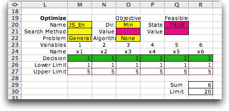
A form is constructed by the
add-in and is shown below. We call this the combinatorial
form because we use it to optimize the discrete variables
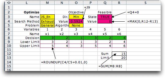
in combinatorial problems. In the second figure several of
the cells have been changed from their initial values to
represent the example.
Initial Form
Form after modifications
|
| |
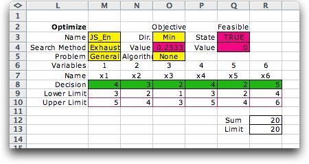
The form has 6 columns for the
variables holding the values and lower and upper limits for
the combinatorial search. We have placed formulas for the lower
limits that compute the minimum number of channels for each
station. We arbitrarily make the upper limits 2 greater than
the lower limits. The value cells in row 8 are colored green
to indicate that the program will manipulate these values during
the search procedures. Cell M3 holds the name, cell M4 holds
the search method that may be changed later, the Problem type
appears in M5. We use the General type for the range
problem. Cells colored yellow hold information manipulated
by the add-in and should not be changed by the user.
Cell O4 holds the direction of optimization and cell O5 holds
the formula for the objective function. In this case the formula
is simply "=J9", where cell J9 holds the value of
the mean time in the system for the queuing network. The cell
is colored pink to indicate that the user must provide the
formula that links the model to the combinatorial form. Cell
O5 does not play a role in this example. When appropriate,
this cell will hold the name of a VBA subroutine that is called
as part of the evaluation process. For MIP, network or transportation models
it will hold the names LP/IP, Network or Solver. For layout problems
cell O5 holds the name of the layout solution subroutine.
We have added cells R12 and R13 to describe the constraint
on the total number of servers. R11 computes the total as the
sum of the values in row 7 and R12 holds the upper limit. Cells
R12 and R13 are not part of the combinatorial form, but were
added after the form was constructed. Cell Q4 is created by
the add-in to hold a Boolean expression that indicates whether
the current solution is feasible. In other situations this
cell can use very complex computations to determine feasibility,
but in this case we want the cell to indicate TRUE (feasible)
whenever the total number of servers is less than or equal
to 20 and FALSE (infeasible) otherwise. The easiest way to
do this is by the logical expression:
=Q4=0
This expression returns TRUE whenever the contents
of cell Q5 is 0, and false otherwise. The add-in uses the cell
Q5 to provide a numeric measure of infeasibility. In this case
we place in Q5 the expression:
=MAX(0, R11-R12)
This expression is 0 for feasible solutions and positive for
infeasible solutions.
The next important step of preparation is to link the variables
of the queuing model with the variables on the combinatorial
form. To do this we place formulas for the Number of Servers that
link the enumeration variables to the model variables. This
is easily accomplished by typing "=M7" in cell C6
and using fill right for the remainder of the row. |
| |
|
Exhaustive Enumeration |
| |
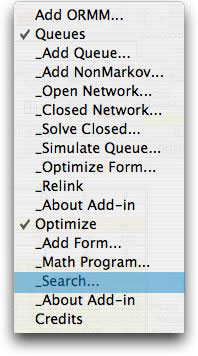 |
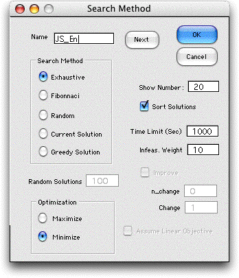
To initiate the search, we choose Search from
the menu. The dialog below is presented. The program places
the name of a combinatorial form on the active worksheet
in the name field. If there is more than one form on the
worksheet, use the Next button to cycle through
them. The buttons in the search method area select the
method. For the example, we have chosen to enumerate all
the solutions within the range.
|
|
| |
The program will show the best
solutions encountered during the enumeration in a list on the
worksheet. Select the desired number in the field provided
and click the checkbox if you want them sorted by objective
value. At the end of the time limit specified, the
program will stop and ask if the process is to continue. Since
the enumeration time may be very large, it is good to have
this opportunity to terminate the run. The infeasibility
weight is not important for exhaustive enumeration, but
it plays a role in the other search methods.
After clicking OK, the program computes an estimate of the
number of solutions and shows it on a dialog. The user may
wish to terminate the process if this number is too large.

The results of the enumeration
are shown below. The program places the variable values for
each alternative in row 8 and evaluates the solution. A total
of 729 solutions are generated. For those that are feasible,
the objective function is computed. At termination, the optimum
number of servers is displayed in green cells of row 8.
It is important to note that the add-in controls the enumeration
process and generates the values of the decision variables.
The objective value and feasibility value and state (cells
O4, Q4 and Q3 for the example) are computed by arbitrary formulas
placed on the worksheet. There are no restrictions on the worksheet
model, so the add-in makes no assumptions about linearity or
other mathematical characteristics. It is necessary that the
objective value and feasibility value and state be computable
for at least some of the values of the decisions. Otherwise,
the process might be interrupted by an Excel error message. |
| |
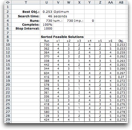 |
In addition to the optimum, a sorted list
is placed to the right of the combinatorial form. For the
example, the 19 best solutions encountered are shown on
the list. The optimum is recomputed at the end of the run
and is shown as the 20th solution. The list is often valuable
when there are non-quantitative aspects of the problem
that would suggest the use of a solution different than
the optimum.
The example required 46 seconds on the author's computer.
The time is proportional to the number of evaluations and
the time required for each worksheet computation. The latter
depends on the complexity of the worksheet model and the
speed of the computer. For the queuing network, there are
a number of user-defined functions involved. These take
much longer to evaluate that Excel formulas or built-in
functions. |
|
| |
Exhaustive enumeration is a very
general procedure for combinatorial optimization. There are
no restrictions on the format of the objective function other
that it be computed by an evaluation of an Excel worksheet
or VBA subroutine. Issues such as convexity or continuity are
irrelevant and the global optimum solution is always obtained
if the process is run to completion. Of course the difficulty
with this approach is the exponential growth in the number
of solutions with the number of variables and the width of
the range for each. Nevertheless many practical problems have
low dimensionality and exhaustive enumeration can play an important
role.
The other search alternatives may require less computation
time but no longer guarantee optimality. |
Feasibility |
| |
Feasibility plays an important
role for many optimization problems. There are two kinds of
infeasibility. First a feasible solution must have each of
the variables within the ranges specified by the upper and
lower limits on the variables (rows 9 and 10 for the example).
The exhaustive generation procedure does not generate solutions
that fall outside these limits, so keeping the feasible range
as small as possible is important to reducing the time of enumeration.
The second kind of infeasibility is represented by the Boolean
expression in cell Q3. The contents of this cell can be the
result of many complex feasibility conditions. When the cell
evaluates as TRUE, the solution is feasible and its objective
function is compared with the objective values of other feasible
solutions. When the cell evaluates as FALSE, the solution is
infeasible and disregarded. Although this feasibility test
can be very powerful and important to modeling, it does not
reduce the number of solutions that are generated.
The value in cell Q4 measures the amount of infeasibility
for an infeasible solution. This cell is not important for
exhaustive enumeration unless it determines the value of Q3,
as it does in the example. The formula for Q3 could have been
easily written so that it not depend on Q4. Then the contents
of Q4 would have no effect on the process. |
| |
|
|


