|
|
Activities in a project require
the expenditure of cash and may involve the receipt of
revenues. The add-in models the inflows and outflows of
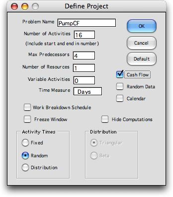
cash with the Cash
Flow feature. The cash flow data and analysis is included
by clicking the Cash Flow checkbox in the Define
Project dialog. We continue with the pump installation
example described earlier, but now include cash flow data.
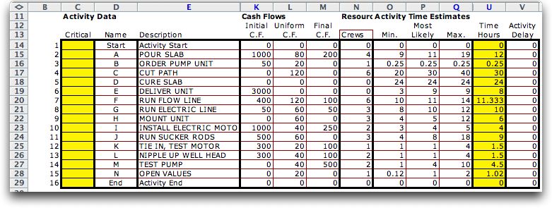
The data form below includes columns defining the cash
flow for each activity. The figure below shows part of
the worksheet with the cash flow data. The columns holding
the precedence relations as well as the columns computing
the mean and standard deviation are hidden. The times in
column U are the mean activity times.
Our models
use three cash flow quantities for each activity. The Initial cash
flow occurs when the activity begins. This would model
the cost of purchasing materials and setting up equipment.
The Uniform cash
flow is expended for each unit of time the activity progresses.
This would model the labor costs and equipment rental
costs, measured in cost per unit time. The Final cash
flow occurs at the time the activity is complete. This
might model the cost to perform tests and to disassemble
and move equipment. We have estimated these costs for example
in the table below. The Uniform cost is the Crew size
multiplied by $20 per hour. |
|
| |
| |
Although we have
used only costs for the example, the project might involve
revenues as well. It may be that some activities provide income
through sales or rental receipts. Other activities may require
an initial investment but part of that investment would be
returned as salvage when the activity is complete. The model
assumes costs are positive numbers. Revenues
would be shown as negative numbers in the table.
The provision of variable time
activities described on a later page allows additional
interesting model variations. |
|
| |
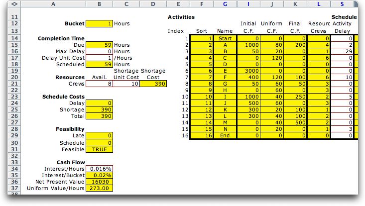
The data for cash
flows is stored on the Project Definition worksheet,
but the cash flow affects the Schedule worksheet.
A portion of the schedule worksheet showing the cash flow
components is shown below. The scheduled start and finish
time are for the early-start schedule. Again some columns
are hidden. Columns I, J and K hold formulas that link the
values in these cells to the data on the definition worksheet.
The cash flows for the Start and End
activities are all zero. |
| 
|
| |
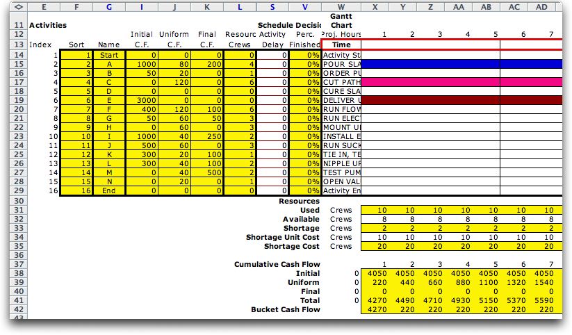
Below we see part of the Gantt
chart for the schedule. The current time is 0. The rows immediately
below the chart compute the resources used by the schedule and
the shortage costs incurred. For the example, we are using 8
crew members with a shortage cost of $10 per hour. This is the
penalty for paying an overtime crew person $10 more per hour
than the normal time $20 per hour. Rows 38 through
41 show the initial, uniform, final and total cash flows for
each bucket of time. In addition to the uniform cash flow for
each ongoing activity, row 39 includes the shortage cost. (This
is a change from earlier versions of the add-in.)
Row 42 computes the total cash flow in each bucket. The
values are all computed automatically with Excel logical and
mathematical functions. The table continues to the right for
as many buckets as required by the schedule. Because of the
discrete time buckets, the uniform costs will be approximate
if activity times are not integral multiples of the time bucket
interval. This is the case for the example because the activity
times have fractional components. |
|
| |
|
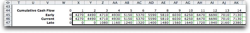
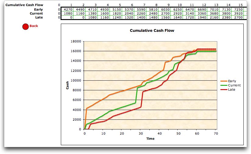
Clicking the Cash Flow button
at the top of the schedule worksheet computes the cash
flow for three schedules: the schedule with the activities
beginning at their Earliest start times, the
schedule currently specified on the worksheet, and the
schedule with the activities beginning at their Latest
start times.
The three results are shown starting at row 45. Only
the first few buckets are shown with the table continuing
to the right. Since our example uses the early time
schedule, the Early cash flows are the same
as the Current cash
flows. These results are shown with green borders because
they are the result of an algorithmic calculation and
are not dynamic. If the schedule changes or any data
changes, the table must be recalculated by clicking on
the Cash
Flow button. |
|
|
| |
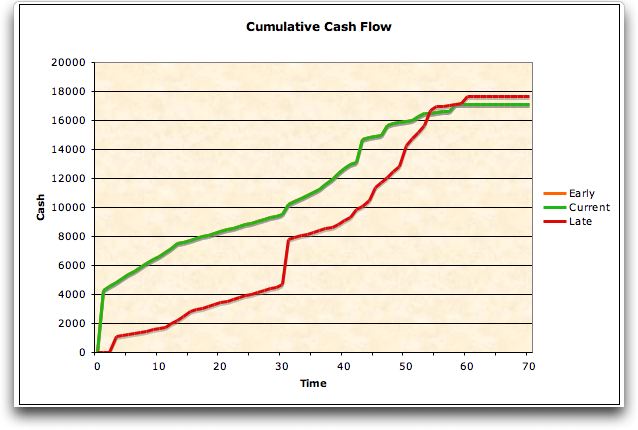
The cumulative cash flows
are shown in a chart as below. When there are no resource shortages
, the Early
cash flow will be to the left of the Current and Late
cash flows. Similarly, the Current cash flow will be
to the left of the Late cash flows. When there are resource
shortages, the curves may cross. For the example,
the Late cumulative
cost ends at a value slightly greater than the Early cumulative
cost because the latest schedule has more costs. The discrete
time buckets may also cause minor inaccuracies. |
|
Results |
| |
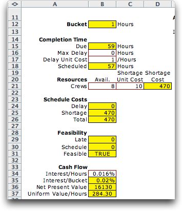
When cash flows are
defined additional results are computed in the first few columns
of the schedule worksheet.
|
The rows through row 31
hold results previously described. The particular results
shown here were obtained for the early-start schedule.
The assumed shortage cost is in C21.
The cash flow results start in row 34. Since the cash
flow is a series of time-bucket cash
flows, a reasonable measure of
the cash flow is its net present value. The data in cell
B34 is the interest rate or discount rate
for the net present value computation. When the bucket
is not the same as the time interval, the interest rate
must be adjusted for the bucket time interval. That
computation is in cell B35. Cell B36 computes the net
present value for the bucket cash flows starting in
cell X42 in the figure above. The computation uses an
Excel financial function. For the example we use a discount
rate of 0.016% per hour. This roughly corresponds to
25% per year.
A better measure for comparison is the Uniform
Value computed in B37. This cell is computed
with an Excel function using the interest rate in
B34, so it is the cost per unit time (per hour in
the example). We use this measure for the search procedure
described below. |
|
Search |
| |
With cash flow analysis,
there are several different options for the search process.
Initiate the search process by clicking the Search
button at the top of the page.
The search options are presented in the dialog below. We discussed
most of this dialog earlier. Clicking the Min. Cash Flow option
selects the Uniform Value, computed in B37, as the
objective to be minimized. Clicking the Min. Schedule Cost minimizes
the shortage cost in B26, thus neglecting the cash flow.
When the Transfer the box at the bottom of
the page is checked, the delay column associated
with the search solution is transferred to the Project worksheet.
The transfer can also be accomplished by clicking the Transfer
Schedule button
at the top of the page.

After a few seconds, the add-in returns the message
that the uniform value has been lowered by 40.5.

Regardless of the objective, the search process uses the same
heuristics as discussed previously.
Since there are no revenues in the example, minimizing the
uniform value tends to move the start times later. The completion
time has been delayed to 59. The scheduled delays are increased
for several activities. |
|
| |
The cumulative cash
flow chart shows the results for the search solution as the
green line. For most of the time horizon, the search solution
spends money earlier than the early-start solution, but sooner
than the late-start solution. We should note that the cumulative
cash flow chart is not dynamic. Any time a solution is changed,
you must click the Cash Flow button to obtain a new
chart.
|
|
| |
Incorporating cash
flows into the analysis extends considerably the kinds of questions
that can be posed and answered with this Project Management
add-in. The next page introduces Variable Time activities.
These can be very useful when considering project cash flows. |
| |
|