Alternatively, it may be desirable to find a schedule the provides a uniform level of resource usage. Here we would like to minimize the variance about the mean usage or some other specified quantity. Here the goal is Level the resource.

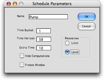
Our optimization routines may use either measure, but their calculations depend on the one chosen. On this page we show how each measure is calculated. Select the resource treatment by clicking a button on the schedule dialog.

The model for resource usage requires 0-1 variables that indicate whether activities are active or not. An activity is active if it has started, but not yet finished. We define this variable in terms of time buckets used for scheduling. It is easiest to think of a time bucket as one unit of time.

To see how the values of the activity variables are computed on the Schedule worksheet, we eliminate the formatting from the first 20 periods of the Gantt chart in the figure below. The cells starting in column U all have the same logical expression:

=IF(AND(Pump_SchedStart<Pump_T,Pump_SchedFinish>=Pump_T),1,0)

The name Pump_SchedStart refers to the scheduled start times in column Q.

The name Pump_SchedFinish refers to the scheduled finish times in column Q.

The name Pump_T refers to the time indices in row 13.

The expression evaluates to 1 during the periods when the activity is active, after it starts and before it finishes. These cells are used to evaluate resource and cash flow usages during the time for the project. As the schedule changes, the locations of the 1 values in the Gantt chart move to the right or left.

We define notation for resources.

We compute the resource usage and the cost of excess usage using the following.

Resource usage is calculated on the worksheet using the SUMPRODUCT function. Each entry in row 32 is computed with a similar formula. The formula below is for cell U32.

=SUMPRODUCT(U14:U29,Pump_Res1)

The name Pump_Res1 refers to the resource requirements in column I.

The range U14:U29 refers to the activity variables for time 1. In the Gantt chart pictured above, to find the crew requirement for time 1 multiply the column for time 1 by the column for the activity crew requirement. The product determines that a crew of 6 is used for period 1. These are used for activities C, cut path, and E, deliver unit, that are in process. C requires all 6 and E requires 0. Since the limit for crew size is 8, the slack for this period is 2 and there is no shortage. The shortage is computed in U33 as 0. At time 5, activities A (pour the slab), C and E are in process requiring a crew of 10 (cell Y31). The shortage in Y33 is 2. The unit cost in X34 is 1, so the shortage cost is computed in X35 as 2.

When the worksheet is created, all the resource availabilities are linked by equation to cell B8, holding the value 8, and all the shortage costs are linked to C8, holding the value 1. Changing these two cells changes all cells in rows 32 and 34 respectively. In practical situations resource availabilities and costs will change over time to represent weekends or holidays. The appropriate cells can be adjusted by hand or using Excel formulas to provide this variation.

Level Model

For this model we choose the Level button in the schedule dialog.

For the level model we want to minimize the variation of resource usage about the amount of the resource available. The objective reflects the goal of having a uniform amount of the resource used during the life of the project without great variations above or below the amounts available in the different periods.

The mathematical development is below. The variation of the resource depends on the schedule through the x variables and the amount of variation is represented by the s variables. The variation in any one period may be positive or negative, but the squared value used in the evaluation is always positive. As for the limit model, the amounts available (R) may vary over the periods in T. Although we allow the cost of variation (c) to vary over time and resource, for most cases it would be appropriate to use 1 for all values.

An interesting observation occurs if we say that the amount of the resource is constant over time. In the following we assume all variation costs are 1 and that the resource available (R) does not vary with time. We expand the squared term

In the final expression for the cost of variation we identify two terms using the large brackets. The first is a constant that does not depend on the schedule. The second term does depend on the schedule and is the sum of the squares of resource usage over time. For optimization, any constant term can be neglected without affecting the optimum solution, so the optimum only depends on the sum of the squares of resource usage. The values used for resource availabilities (R) do not affect the optimum solution when the goal is to minimize the cost of variation.

This result is not true if the resource availability changes over time. The analysis also depends (in the second line from the bottom) on the fact that the total time required for each activity, and thus the total resource required, does not depend on the schedule. This is not true if some of the activities using resources are variable time activities.

The analysis also assumes that the time required for the project (T) is constant and does not depend on the schedule. This is not true if the optimization allows the total time to change with the schedule. If we allow the time to change, it may be possible to reduce the sum of the squares by spreading out the project into more periods. This may or may not reduce the total variability or the average variability in time. We do not adjust the analysis for this because it is unlikely that the project duration will be allowed to extend many periods beyond the due date. The resultant approximation is small.

When variability is more important for one resource than another, the cost parameters (c) many be different for different resources. This does not change these results unless the costs vary over time.

The figure below shows the Gantt chart when variance is the measure to be minimized. Rows 31 and 32 show the amount used and available in each period. Row 33 shows the difference between the amount used and the amount available squared. The variance cost is evaluated in row 35. Since the unit cost is 1, rows 33 and 35 are the same. When there is more than one resource, rows are provided for each.

The variance summed over all periods is shown in the results section at the left side of the worksheet.

Optimize

To optimize the schedule we click the Search button at the top of the page. For the objective we choose to minimize the schedule cost. For this example, we will generate 50 random solutions and improve each one.

The results of minimizing the variance are shown below.

This is quite a different schedule than that obtained earlier. The resultant schedule is shown in columns Q and R. There is no guarantee that this solution is optimal. The methods used are direct search procedures that vary the delay times while attempting to reduce the objective function. Of course, using more random starting solutions will give more confidence in the results, but heuristic methods can never guarantee optimality.