Population	1000 Simulations

Project management results depend on many random variables. In these models we assume that all activity durations are independent random variables, so to simulate the project we simulate every activity and observe the results obtained. For any one simulation replication, there is a critical path and the length of the critical path determines the completion time of the project and whether the project satisfies the due time or not. With a number of simulated replications, the simulation gathers data about each result and finally presents the results in tables. We illustrate the process below.

The model to be simulated is the description of the project on the Excel worksheet. The worksheet using the triangular distribution for activity durations is shown below. Simulation is initiated with the Simulate button at the top of the page.

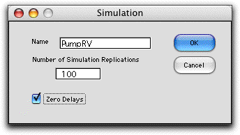
The Simulation button presents the simulation dialog shown below. It includes a field to enter the number of replications for the simulation and a button indicating whether to zero the delay column or not. Making the delays all 0 will give the greatest flexibility for scheduling, however, there will be cases where it is better to leave the button unchecked. Then the delays remain fixed as they are when the simulation was called.

The add-in replaces the times in column N for the example, with a function from the Random Variables add-in. For the case of activity A the cell N15 holds:

=RV_SimV(G15:J15)

This function performs a Monte Carlo simulation for the distribution described by its arguments. For activity A it is a triangular distribution, (G15), with lower limit 9, (H15), mode 11, (I15) and maximum 19, (J15).

Although the functions in column N are the same except for the relative references, so each returns a single number that is the simulated value of the random variable.

Simulation Results

The Excel model defining the project computes the critical path for the simulated times. The add-in accumulates arrays holding the number of the replications in which each activity is critical, the total completion time and the number of replications where the completion time satisfies the due time. The averaged results are shown in the table below the project definition.

It is interesting to compare the simulated results with the critical path determined with the mean values of the activity times (shown in red below). All but two of the replications had the same critical path. The mean critical path length time computed as the sum of the activity means (61) is about the same as the simulated value (61.05), and the variance and on-time-probabilities are also about the same.

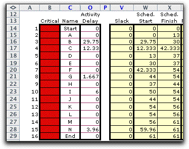
A different result occurs when we choose to start each activity at the latest possible time. The settings for this case are below. Each activity is delayed as much as possible and all slack values are 0. The project is completed at the same time (61) when considering only the length of the longest path.

When we simulate this case we choose not to zero the delays by leaving the box unchecked. Zero delays give the early start solution.

The simulation results show that every activity is in the critical path of some of the 100 replications. The mean simulated completion time (65.28) is quite a bit higher than the length of the longest mean path (61) and the variance (9.86) is smaller than the case when all activities start at the earliest time (20.5). The variance shown in the approximate results on the right are not really valid since it is the sum of the variance of all critical activities. Assuming the mean times, they are all critical, but for any replication, only a subset are critical. The simulated probability of meeting the due date (0.02) is almost 0.

Simulation with Advanced Time

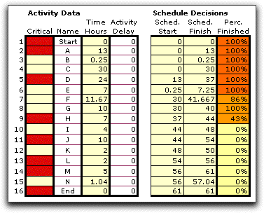
Once the project begins and time progresses, some projects are completed and others are in progress. The simulation only simulates those times for activities not yet finished. For the example we advanced the time to 40. Activities A through E are finished. Activities F through H are in progress (G is just finishing). Activities I through J are not started.

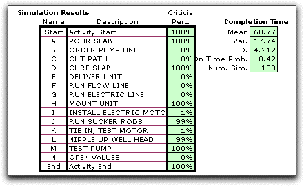
The simulation fixes the values of the times for those activities already finished and simulates the remainder. As time advances, the results should show less variability, because the times for activities already finished cannot vary. This is illustrated by the example below that fixes the time for activities A through E.

When evaluating the simulation method we must review some of the abstractions necessary to do simulation. Most are embedded in the abstractions used for the project model itself. Every replication assigns specific times to the activity durations and computes the critical path and the associated project completion time with the critical path formulas. These formulas are placed directly on the worksheet and are dynamically computed for each replication. The simulated times however are not random variables, they are single values, just as would be obtained when the project is actually performed. If the model is correct, each replication yields a result that could be observed in reality. If the model is correct, reality is just another replication of the model.

One assumption of the simulation model that was not stressed previously is that the random variables representing the different times are independent. Each activity value is selected independently of the rest.

Simulations are better that the mean value model used to this point because it explicitly represents uncertainty. The careful Excel modeler who knows that the inputs to his model are inherently uncertain will use trial and error to see how the results vary with the inputs. Thereby the modeler tries to determine if the results are sensitive to input variations. Simulation is essentially an automated what-if experiment that can be performed many times. The simulation results show the sensitivity of the solution to the inputs that are simulated. For the example with early starts, we see that the identity of the activities on the critical path are not sensitive to the times drawn from the given distributions. When the late start assumption is used, the critical path is very sensitive to the times. Simulation results can be made as numerically accurate as necessary by using more applications. A run of 1000 replications takes very little longer than 100 replications.

Of course if the model is not correct, the results will not be realistically accurate. This is surely the case since any model is an abstraction of reality and the results are never the same as would observed in reality. This does not mean that the results are useless. The simulation points out activities that are surely critical, others that might be critical and others that are not. This information should be useful to the manager for purposes of focusing his or her attention on the activities that must be performed promptly. The real question is does the model and the method applied to it yield results that are useful in practice? If it does not, the model needs to be modified or discarded. Of course, if it is discarded, the manager must go elsewhere for help.

One feature of the model is not always important. It is often not necessary to know the exact form of probability distributions. As long as the variability of reality is modeled in some way, the results may not be too dependent on the exact features of the distributions. Of course one always test this hypothesis with the Excel model.