|
|
 |
Project
Management |
 |
-
Uncertainty |
 |
Uncertainty is an inherent aspect of project management. When
the model is constructed and the critical path is determined,
all activities are future events. Inputs to the project management
analysis include for each activity estimates of the time duration,
estimates of resource usage and estimates of costs. Of course
there may also be uncertainty with regard to the activities
that comprise the project and the precedence relations that
relate them. In many cases everything about the project is
to some extent uncertain, but on this page we consider only
the uncertainty of the time durations of activities.
There are many kinds of uncertainty, ranging from "I
have no idea" to "I can estimate probabilities about
uncertain quantities." We use the latter case, which
is sometimes called risk. We assume that although activity
durations cannot be known with certainty, we can provide probability
distributions that indicate the likelihood of various values.
For a discussion of probability see the article in the ORMM/Supplements/Models/Probability
section. The PDF document about Continuous
Probability Distributions is particularly relevant.
In a project environment, all uncertainty will eventually be
revealed, assuming that the project is actually finished. The
revelation occurs as time passes and as activities are started,
performed and finished. If times, resource use and costs are
recorded, the project manager will know how the project is progressing.
At times after the project has begun but before it is complete,
the manager may take action to change all features of the model
that are not yet completed, make new analyses and take corrective
action where appropriate. Project management is far more than
determining the precedence relations, estimating resources and
costs and computing the first critical path. Estimates made
before the project begins must surely be adjusted to account
for the reality of results. The ability to make adjustments
after the project has begun partially helps with the problem
with uncertainty. Plans can change. Decisions may shift as the
future is revealed by the passage of time. |
Probability Distributions
|
| |
There are many human
and political factors that bring to question the time estimates
provided by persons associated with a project. We will not discuss
them here, but there is a good discussion in the book Critical
Chain by Eliyahi Goldratt (North River Press, 1997).
Putting the human and political issues aside, the duration
of something that has yet to occur is at best a random variable.
It cannot be known with certainty. Construction projects depend
on weather, labor and material availabilities, all of which
can affect activity duration and cannot be accurately assessed.
Projects involving creative effort such as software development
depend on the intellect and insights of the participants,
certainly difficult to predict. The remainder of this page
and the next will consider the effects of uncertainty using
continuous probability distributions. The treatment of the
times as random variables is an explicit recognition of uncertainty.
The CPM model, using only one estimate, completely neglects
the effect. PERT with three estimates, recognizes uncertainty,
but does not prescribe probability distributions. This makes
it impossible to use the results of probability theory except
in an approximate way or to use simulation as part of the
analysis. Simulation is considered on a later page.
| |
To use probability distributions, the Random
Variables add-in must be installed in Excel.
This add-in provides access to sixteen named probability
distributions as well as user defined and simulation generated
distributions. Functions provided by the add-in compute
moments, such as mean and variance, compute probabilities
and inverse probabilities and perform Monte-Carlo simulation.
Many of these are used by the analysis on this and the
next page. It is not necessary for the user to be well
versed in the use of this add-in or in probability theory,
because the Project Management add-in performs
the interaction. The Random Variables add-in
must be installed, however. If properly installed, the
menu items on the left will appear under the OR_MM menu.
Although it is not necessary to use these menu items,
the Relink Functions command will be useful when
opening workbooks that contain RV functions created
on other computers, such as the Demo workbook downloaded
from this site. Simply select the Relink Functions
command to replace the functions with those created on
your computer. |
The triangular and Beta distributions are the most often used
in project management studies because both can be characterized
by the minimum, most likely, and maximum parameters. As we will
see later, other distributions are also available.
The triangular distribution is used in our first example.
An illustration of the triangular distribution is below. The
example has a minimum of 0, a most likely value (or mode) of
0.3 and a maximum of 1. The distribution is shown by the heavy
line and the cumulative distribution is shown by the dotted
line. Triangular distributions with other parameters are shifted
and/or spread out. The area under the distribution curve is
always 1. The cumulative distribution shows the probability
that the random variable is less than the value given on the
horizontal axis. For the example, the probability that the random
variable is less than 0.4 is about 0.5. In general this is called
the median. The mean of this example is 0.433.
If this were an activity time distribution, project management
analysis will use the mean value of 0.433 as the single time
estimate for the activity time. The variance is also
used for the analysis, and for the example pictured, the variance
is 0.0439. The mean and variance values are computed by the
Random Variables add-in. The figure below was constructed
by the add-in.

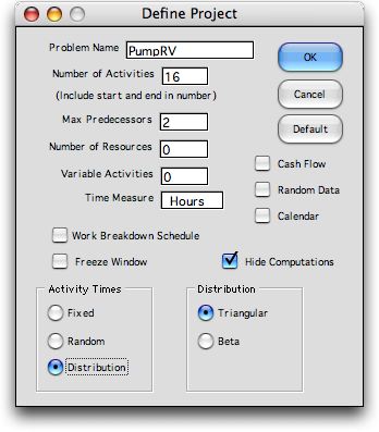
To create a model with random activity times click the Distribution
button in the Activity Times frame of the definition
dialog. Two distributions are available in the Distribution
frame, Triangular and Beta. We use the Pump
example considered earlier, but now the activity times will
have triangular distributions.
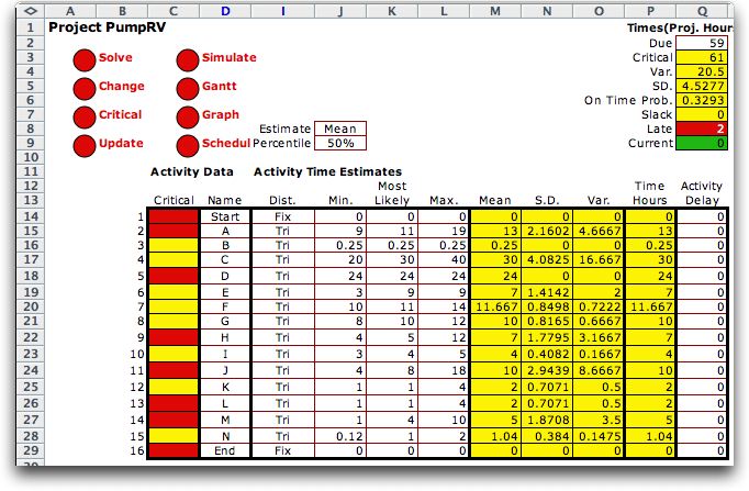
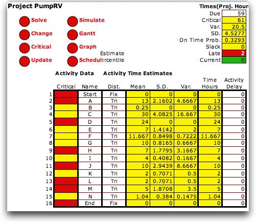
The worksheet model is constructed as below. We
have hidden some columns to simplify the explanation. We provide
only two columns for predecessors and use no resources for this
example. The model has already been solved and the critical
activities are colored red in column B. The critical predecessor
relations are colored green in columns E and F. The mean values
computed for the triangular distribution are used in the Time
column (N). The only apparent difference in this worksheet and
the worksheet for the traditional model is the column containing
the letters "Tri". These letters identify the triangular
distribution. The letters "Fix" specify a fixed or
constant distribution for the start and end activities. |
|
| |
It is interesting
to compare the results with the triangular distribution with
the results using the traditional PERT formulas for computing
mean and variance. We show below the columns with mean and variance.
The distribution parameters are as above. The triangular distribution
results are on the left and the traditional results are on the
right. The mean and variance values for the triangular distribution
are computed by functions provided by the Random Variables add-in.
As expected, the mean, variance and standard deviation values
for each activity are different because the traditional analysis
uses empirical formulas for computing these quantities and the
Random Variables add-in computes the accurate values for the
triangular distribution. Since, the activity times used for
the analysis are the mean values, the results shown at the top
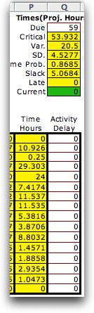
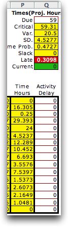
of the page are different for the two cases. In both cases we
choose the due date of 59. The critical path, which is the same
for both cases, has an expected value of 57 for the traditional
method and the project has a slack of 2. For the triangular
distribution, the critical path has an expected value of 61
and the project is late by 2. The variance and standard deviation
values are also different leading to a different estimate of
the standard deviation for the project. Of course the probabilities
of completing the project by the due date are quite different. |
| Triangular
|
Traditional

|
|
| |
Which analysis is more
accurate? Probably neither is accurate. The estimates of the
parameters are usually the biggest source of error and the assumption
about probability distributions less important. Although the
traditional analysis is unclear about the distribution, there
is really no reason to believe the triangular distribution represents
reality. The example does point out that the numerical results
such as the expected value of the critical path and the probability
of meeting the due date, are sensitive to distribution assumptions
and are thus suspect regarding validity. The principal value
of using a known probability distribution is that Monte-Carlo
simulation is then possible. Analysis with simulation may lead
to useful results as described later.
Another distribution often used for project analysis is the
Beta distribution described on the next page. |
Time Estimates |
| |
To this point an activity
time has been estimated using the mean value of the probability
distribution. We see the figure below the columns representing
the distribution parameters in columns J, K and L. The
distribution means, standard deviations in columns are computed
in columns M, N and O. The estimates of the activity times in
column P are the same as the distribution means. Cells Q3 computes
the sum of the means for the activities on the critical
path. Cell Q4 computes the sum of the variances for the
activities on the critical path, and Q5 is the square root
of that value. Assuming the normal distribution for activity
times, cell Q6 computes the probability will be completed before
the due date.
The times in
column P are point estimates of the activity times. They
are important because they are used for all the other analyses
on the project worksheets. We have used the mean for the point
estimates, but other point estimates are possible. Cell J8
holds the identity of the point estimate, Mean, for
the example. |
| |
|
| |
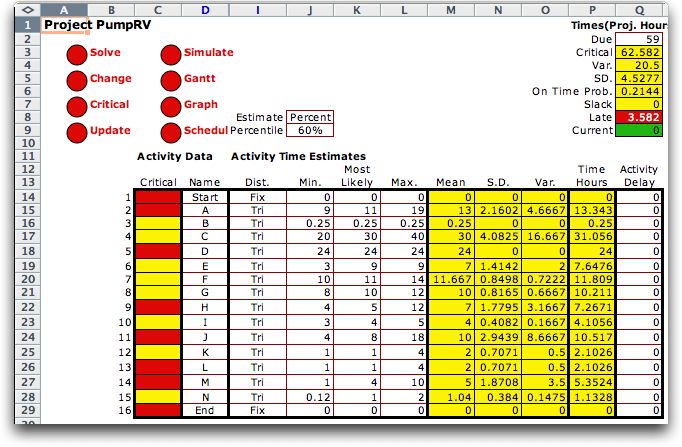
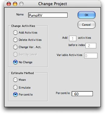
To change the point
estimate, click the Change button at the top of the
page. The change dialog shows the two other options, Simulate and Percentile.
We choose the latter first and indicate a 60% as the percentile
level.
|
| |
The change is reflected
in J8 and J9. Now the estimates in column P are the 60% values
of the distribution. The individual activity times and the length
of the critical path are longer with these estimates. This estimate
may be appropriate if the manager wants a conservative estimate
of the project completion time. |
| |
|
| |
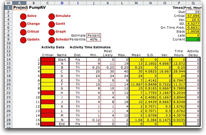
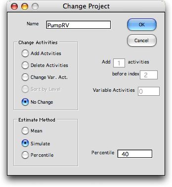
To change the percentile,
simply change the number in cell J9. The figure below shows the
40%-percentile estimates. The activity durations and the critical
path are reduced. These would be optimistic estimates. |
| |
|
| |
The third kind of
estimate is the simulated estimate. The percentile has no meaning
in this case.
|
| |
The numbers in column
P are not simulated from the distribution with the Monte-Carlo
method. |
| |

|
| |
Each time the worksheet is recomputed, the times
are simulated. The length of the critical path is identified
as a random variable because it changes with each simulation.
|
| |
Simulation is not good
for estimating resource usage or cash flows, but it is good
for estimating the likelihood that the individual activities
are on the critical path. We use it on the Simulation page
of this discussion. |
| |
|
|