Computation Section
Project Management
 - Beta Distribution

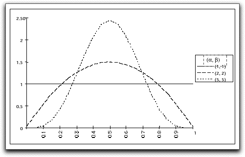
The add-in provides the Beta distribution as an option for the probability distribution. Beta distributions are useful because they are defined between a minimum and maximum value, many different shapes are available depending on the parameters chosen, and, for some parameter choices, the distribution has a well defined mode (most likely point). The distribution has four parameters, alpha, beta, minimum and maximum. The picture below shows three examples of symmetric Beta distributions. For symmetric distributions alpha and beta are the same. As their values increase the distributions become more peaked. The uniform distribution has alpha and beta both equal to 1. This does not have a well defined mode because every point has the same probability. Distributions with alpha and beta less than 1 are bathtub shaped curves and are not useful for modeling activity times.


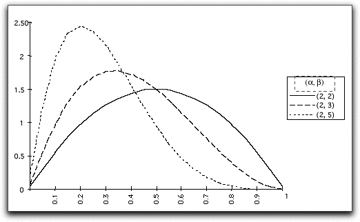
Asymmetric distributions are obtained by choosing alpha and beta to be different. The picture below shows several cases with alpha held constant at 2. The greater the difference between alpha and beta the greater the asymmetry. The asymmetric examples are all skewed to the right because alpha is less than beta. To obtain distributions skewed to the left choose alpha greater than beta.
The generalized Beta distribution has a range other that 0 to 1 and has the extra parameters defining the minimum and maximum. The generalized Beta distributions look the same as the pictures above but are spread out and/or shifted.

The notation for the generalized Beta distribution and equations for the mean, variance and mode (or most likely value) are shown below. The mode is interesting to project analysis, because it is used as a parameter in the traditional analysis.

It is interesting to compare this with the traditional PERT method for calculating the mean and variance. Here the mode is a parameter. The Beta distribution allows much more variety for the variance of the distributions.

The table below shows the mean, variance and mode values for the five different Beta distributions pictured above and compares the results with the traditional calculations of the mean and variance. All have the range 0 to 1.

Alpha
Beta
Mean
Variance
Mode
Trad. Mean
Trad. Var.
1
1
0.5
0.083
***
***
***
2
2
0.5
0.050
0.5
0.5
0.028
5
5
0.5
0.023
0.5
0.5
0.028
2
3
0.4
0.040
0.33
0.389
0.028
2
5
0.286
0.026
0.2
0.3
0.028

There is no mode defined for the uniform distribution described by the first case. For the other cases the traditional variance calculation yields the same result since it only depends on the range. For asymmetric cases, the difference between the Beta distribution mean and the traditional mean increases as the distribution becomes more skewed.

For project analysis we may be given the mode and require values of the shape parameters, alpha and beta, to specify the Beta distribution. Formulas for two cases are below. In each case we must choose one parameter and solve for the other.

When the mode is equal to one of the limits, only one of the equations is valid.


Beta Example


To use a Beta distribution to model activity times, select Distribution for the activity times and click the Beta distribution button.

We have modified the example problem to use Beta distributions for all times except the Start and End activities. Activities B and D are degenerate in that the min and max values are the same. We set alpha and beta to 2 for these cases. For all the other activities except K and L, we set alpha equal to 2 and solved for beta using the second equation above. That equation does not work for K and L because the mode is equal to the upper bound. In these cases we set beta equal to 2 and solved for alpha. It happens that alpha is equal to 1. This is a special case of the Beta distribution that has the form of a triangular distribution.

We solve the problem with the Beta distribution and compare to the traditional results below. We see that the critical path is the same in each case, but the sum of the mean values for the critical path are greater than the traditional resulting in a late project rather than one with slack. The variance for the Beta assumption is also greater, resulting in a smaller probability that the critical path time will be less than the due date.

Beta

Traditional


Other Distributions


The random variables add-in allows several different distributions. They can be used for the project management add-in by simply replacing the name of the distribution and specifying the parameters in the cells immediately to the right of the name. The figure below shows the Beta distribution replaced with other distributions allowed by the Random Variables add-in. We have replaced the titles at the top of columns H through K with general names since the distributions all have different parameters. For the Normal distribution only two parameters are necessary, the mean and standard deviation. These are placed immediately to the right of the name Nor. The remaining parameter spaces are filled with zeros. The complete name could be spelled out, because only the first three letters are used by the add-in, except in the case of the integer uniform and triangular distributions. Review the discussion of the Random Variables add-in to see how the parameters are presented for the various distributions.

The equations in the mean and variance columns refer to the range defining the random variables as illustrated at the bottom of the figure. These functions are user defined functions provided by the Random Variables add-in.

The use of probability distributions may not yield more accurate results than single estimates. They are however, an explicit indication that uncertainty is present.


Return to Top

tree roots

Operations Management / Industrial Engineering
Internet
by Paul A. Jensen
Copyright 2004 - All rights reserved