To apply mathematical techniques to the situation, the problem must be described in more formal terms. To create a model in an Excel workbook, select the New Problem command from the menu. The dialog below is presented. Note that the time measure was inadvertently entered as days rather than hours. This makes the time unit on the illustration graphs wrong in this respect. Rather than try to correct all of the many figures, we use the day measure through the Resources page. On the Cash Flow page we return to the hour measure.

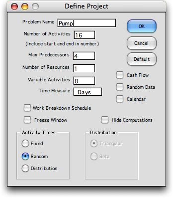
The Problem Name is used to name the worksheet and a number of ranges on the worksheet, so it must be a legitimate Excel name. The name must contain no spaces or punctuation and begin with a letter. The Number of Activities is the number of tasks comprising the project. Fourteen activities describe the project, but we add two more for the Start and Finish activities. The Max Predecessors is the maximum number of predecessor activities for any activity in the project. Although the example requires only 2, we enter 4 to accommodate later changes.

The numbers of persons available to perform the activities of the project is a resource for the example. In general there may be several resources with each activity using a specified amount of each resource. The Number of Resources is entered into the appropriate field of the dialog. The Variable Activities field holds the number of activities that have variable time requirements. We describe this feature on a later page.The Time Measure is hours for the example.

Click the Random Data checkbox to generate a random problem. This is handy for experimentation. Click the Work Breakdown Schedule checkbox to describe the problem with a Work Breakdown Schedule (WBS). The WBS provides levels for the activities so they may be ordered with a hierarchical structure. This structure is described with regard to capital budgeting with the Estimate add-in. The levels option also allows the activities to be sorted based on the level designations.

The Activity Times frame allows times to be specified as fixed quantities (Fixed), represented by three estimates (Random) or described by probability distributions (Distribution) by clicking the appropriate button. We use Random times for the example and illustrate the distribution option later.

hen checked the Hide Computations checkbox hides the columns that hold intermediate information useful for the student, but not immediately necessary for applications. When selected, the Freeze Window option splits the screen so that titles remain fixed while the user scrolls to various parts of the window. This is especially useful for larger problems.

The Calendar options relates project times to calendar dates. We illustrate this on a later page.

The Number of Activities and number of Variable Activities can be changed after the form has been constructed. A calendar can also be added later. All other items on this dialog cannot be changed. Of course it is easy to create a new problem with different parameters.

Worksheet

Precedence and Resource Data

An important aspect of scheduling is that an activity cannot begin before all its predecessor activities are complete. Columns F and G are available to enter this data for the example as shown in the figure above. We have hidden columns H and I because they are not used since there are only two predecessors. Predecessors are indicated by name. Thus we see a predecessor for activity D (Cure Slab) is activity A (Pour Slab). The names in the predecessor range must be exactly the same as those in the name column. It is unnecessary to indicate predecessors for the End activity or to indicate that the Start activity is a predecessor for other activities.

Next to the precedence columns, columns are provided to enter colors for the gantt chart (J), the resource requirements (K) and time data for each activity (L, M and N). For the example, we have a single resource column to hold the crew sizes for the activities. The name of the resource is entered just above the column (K13). This name is used to identify the resource on the Schedule page of the workbook.

Time Data

For the Fixed Time option, only a single data column is provided for the activity time. This is the case for the CPM model.

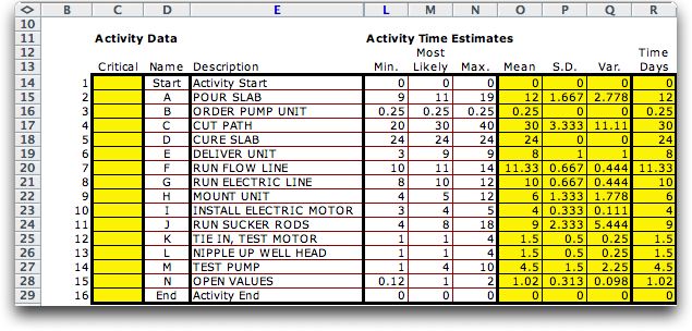
The PERT model assumes that activity times are random variables. For the Random Time option, three data columns, L through N, and four computed columns, O through R, are used as illustrated for the example. Cells for data are white with maroon borders and cells with formulas are yellow. The contents of yellow cells are created by the add-in and should not be changed. The columns representing time estimates are shown below for the example. Columns O through P hold the statistical measures for the distributions. Column R holds point estimates for the activity times. Here the point estimate for an activity is the mean of its distribution.

The traditional PERT model describes a probability distribution for an activity time with three parameters. This is convenient for those unfamiliar with more complex representations of probability distributions. The parameters are the minimum time (a in the formulas below), the most likely time (m) and the maximum time (b). Although these parameters are appropriate for the triangular distribution and Beta distribution, the moments computed below are not accurate for either form. The values of a, m and b are placed in columns L, M and N.

The analysis uses the Mean, Standard Deviation and Variance values of the activity time distributions. These values are computed with the empirical formulas below:

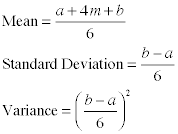
The computations are preformed in columns O, P and Q.

The analysis uses the mean values for activity time estimates, so these values are repeated in column R. This time is used for the critical path analysis. To find the Critical Path for this problem, click the Solve button at the top of the worksheet. The critical path is discussed on the next page.

The add-in also allows the model to use explicit probability distributions by specifying the Triangular or Beta distribution on the problem dialog.

Change

Clicking the Change button at the top of the page allows a variety of model features to be changed. The Change dialog is below. Selecting the Add Activities button, inserts new activities into the model. Activities cannot be added before the Start activity, but any number of activities can be inserted at any other position. For the example we choose to insert a new activity before the activity indexed 2.

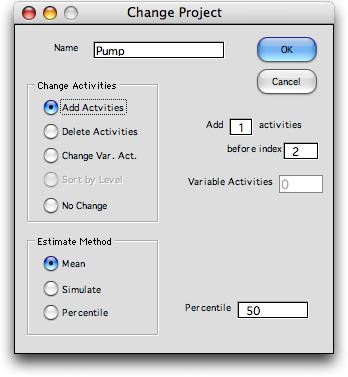
Notice the new activity is named with the letter O. The indices are readjusted to accommodate the new activity.

To illustrate the Delete option, we choose to delete the activity just added.

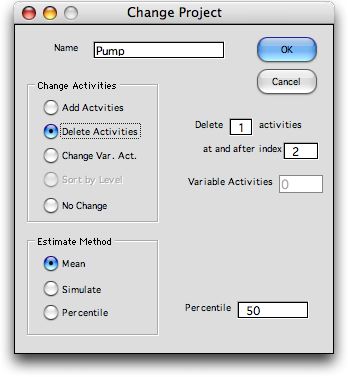
The worksheet returns to the original model. The Start and End activities may not be deleted.

The option is for changing the number of variable activities discussed on a later page.

The change option for the Estimate Method relates to problems that have defined distributions for activity times.

The No Change option is the default selection.

After any change in the model, the formulas determining the early and late times must be regenerated. This is done by clicking the Solve button at the top of the worksheet.