1. The company must rent temporary buildings and other equipment that are to be used for the entire duration of the project. There is a deposit of $500 and the rent is $10 per hour. One employee is hired to work in the office at a cost of $20 per hour. At the end of the project the deposit will be returned.
2. During the process of pouring and curing the slab, special concrete equipment must be rented. The cost of this equipment is $10 per hour. These payments begin with activity A and end with activity D.
3. The company must hire a Registered Professional Engineer for all activities regarding electricity. The requirement begins with the running of the electrical line (G) and ends when the motor is tested (K). The cost of the engineer is $50 per hour. There is an additional paperwork charge of $200 when the engineering is hired.
4. The company will outsource the ordering and installation of the pump unit. The requirement begins with the ordering of the pump unit (B) and ends when the unit is installed (H). There is an initial payment of $200 for this service and a final payment of $300. The crew requirements are reduced to zero for activities B and H, but one person is allocated to this variable activity for supervision. The cost of this person is $20 per hour.
5. In order to finance the project the company will take out a construction loan of $10,000. The money will be received at the start of the project. The company must return to the lender $10,500 at the end of the project. We also include in this activity the management costs for the project of $80 per hour.

These activities are different than those formerly described in that their starting times and ending times depend on the start and end times of other activities and are not fixed. For a variable activity we specify two fixed time activities, a From Activity and a To Activity. The activity described by paragraph 2 above starts at the same time as A (the From Activity) and ends at the same time as D (the To Activity) . When the From activity is left blank, the variable activity starts at the beginning of the project. When the To Activity is left blank the variable activity ends when the project is completed.

For an additional variation, the company receives income for the project. The company will be paid $27,000, to be received in three payments. The first payment of $9,000 will be received at the completion of the slab curing step (activity D). The second payment of $9,000 will be received when the electric motor is installed (activity I). The last payment of $9,000 will be received when the project is completed (the End activity). Three variable activities are added to represent the payments. The variable activities are defined in the table below.

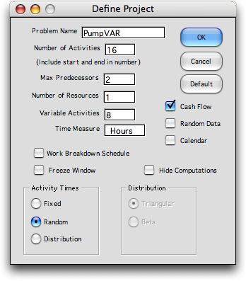
The project is defined using the dialog below. We enter 8 as the number of Variable Activities. The Change button on the project definition page allows this number to be increased or decreased.

The data form for the complete problem is shown below. We have adjusted the cash flow data for some of the activities to reflect the new information. The crew resources for G and H have been reduced to 0 because these activities have been outsourced. The variable activities require some additional crew resources. Costs are represented as positive cash flows and revenues are negative. We have associated the payments with the final cash flows for the activities that determine the timing of the payments.

Since the fixed times have not changed for this example, the critical path and other time-related results are the same as when variable activities were not considered. The variable activities do not affect the early and late schedule, however, they do simplify the modeling of costs and resources when activities span a series of fixed-time activities. These will affect the optimum schedule when costs and resources are considered.

Of course it is important that a variable activity not end before it begins. This illogical result is possible if one chooses a From activity that is not restricted by the precedence relations from starting after the end of the To activity. The program does not check for this, but in most reasonable cases the normal relationships between fixed-time activities will prevent it.

Clicking the Solve button builds the equations that determine the scheduled start and finish times. The example below shows some nonzero delays. They are determined during the scheduling process. The variable activities start and stop based on the From and To activities.

A portion of the Schedule worksheet showing the cash flow components is shown below. Below we see part of the Gantt chart for the schedule. The rows computing resource and cash flow measures include the contributions of both fixed and variable time activities.

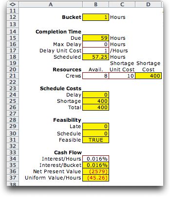
Clicking the Cash Flow button at the top of the schedule worksheet computes the cash flow for three schedules: the schedule with the activities beginning at their Earliest start times, the schedule currently specified on the worksheet, and the schedule with the activities beginning at their Latest start times. The three results are shown in the green field above the graph. Only the first few buckets are shown and the table continues to the right.

The cumulative cash flows are shown in a chart as below. The sudden changes in the cash flow indicates large receipts and expenditures. The last observations on the right shows the cumulative cash flows at the end of the project. These are different for the three cases because the variable activities have different durations for the cases and hence impose different cash flows. The current schedule uses delays to reduce the cost of shortages. The cumulative cost at the end of the time horizon indicate whether the project makes a profit. The cumulative cost for the early time schedule is -1340, indicating a profit of 1340. The profit for the late schedule is 2170, while the profit for the current schedule is 2580.

Results

The results for the current schedule are computed in the first few columns of the schedule worksheet.

The goal of the search procedure was to minimize the entry in cell B37, the Uniform hourly cost. The negative number in this cell indicates that the project returns more than the required rate of return of 0.016% per hour.

Variable activities can be useful for modeling a number of situations that might arise in project management studies. They do not affect critical path analysis, but they may affect the resource requirements and the cash flow. The results are important to scheduling decisions.